  1
  2
  3
  4
  5
  6
  7
  8
  9
 10
 11
 12
 13
 14
 15
 16
 17
 18
 19
 20
 21
 22
 23
 24
 25
 26
 27
 28
 29
 30
 31
 32
 33
 34
 35
 36
 37
 38
 39
 40
 41
 42
 43
 44
 45
 46
 47
 48
 49
 50
 51
 52
 53
 54
 55
 56
 57
 58
 59
 60
 61
 62
 63
 64
 65
 66
 67
 68
 69
 70
 71
 72
 73
 74
 75
 76
 77
 78
 79
 80
 81
 82
 83
 84
 85
 86
 87
 88
 89
 90
 91
 92
 93
 94
 95
 96
 97
 98
 99
100
101
102
103
104
105
106
107
108
109
110
111
112
113
114
115
116
117
118
119
120
121
122
123
124
125
126
127
128
129
130
131
132
133
134
135
136
137
138
139
140
141
142
143
144
145
146
147
148
149
150
151
152
153
154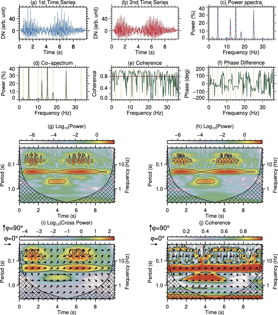
155 | ; pro FIG6__cross_correlation
data_dir= 'Synthetic_Data/'
data1 = readfits(data_dir+'NRMP_signal_1D.fits')
data2 = readfits(data_dir+'NRMP_signal_1D_phase_shifted.fits')
time = readfits(data_dir+'NRMP_signal_1D.fits', ext=1)
restore, 'save_files/frequencies_1D_signal.save'
; cross-correlations: FFT analysis
WaLSAtools, /fft, data1=data2, data2=data1, time=time, nperm=100, cospectrum=cospectrum, phase_angle=phase_angle, $
coherence=coherence, frequencies=frequencies, /nosignificance, d1_power=power1, d2_power=power2, n_segments=2
;----------------------- plotting
colset
device, decomposed=0
walsa_eps, size=[20,23]
!p.font=0
device,set_font='helvetica'
charsize = 1.8
!x.thick=3.2
!y.thick=3.2
thick = 2.0
!P.Multi = [0, 3, 4]
!x.ticklen=-0.080
!y.ticklen=-0.042
df = frequencies[1]-frequencies[0] ; frequency resolution / the lowest detectable frequency
xr = [0,36]
tr = [min(time),max(time)]
; pos = cgLayout([3,2], OXMargin=[10,4], OYMargin=[7,5], XGap=12, YGap=10)
pos = fltarr(4,6)
pos[*,0] = [0.08, 0.8583331 , 0.32111109 , 0.9583331]
pos[*,1] = [0.41111109, 0.8583331 , 0.64888890 , 0.9583331]
pos[*,2] = [0.75888886, 0.8583331 , 0.99 , 0.9583331]
pos[*,3] = [0.08, 0.670000 , 0.32111109 , 0.770000]
pos[*,4] = [0.41111109 , 0.670000 , 0.64888890 , 0.770000]
pos[*,5] = [0.75888886 , 0.670000 , 0.99 , 0.770000]
; --------------------------------
; Plot the detrended & apodized light curve 1
signal1 = walsa_detrend_apod(data1)
cgplot, time, signal1*10., charsize=charsize, pos=pos[*,0], thick=thick, $
xtitle='Time (s)', ytitle='DN (arb. unit)', xs=1, yr=[min(reform(signal1*10.)), max(reform(signal1*10.))], color=cgColor('DodgerBlue'), YTICKINTERVAL=40
xyouts, tr[0]+((tr[1]-tr[0])/2.), max(reform(signal1*10.))+10., ALIGNMENT=0.5, CHARSIZE=charsize/2., /data, '(a) 1st Time Series', color=cgColor('Black')
; --------------------------------
; Plot the detrended & apodized light curve 2
signal2 = walsa_detrend_apod(data2)
cgplot, time, signal2*10., charsize=charsize, pos=pos[*,1], thick=thick, $
xtitle='Time (s)', ytitle='DN (arb. unit)', xs=1, yr=[min(reform(signal1*10.)), max(reform(signal1*10.))], color=cgColor('Red'), YTICKINTERVAL=40
xyouts, tr[0]+((tr[1]-tr[0])/2.), max(reform(signal1*10.))+10., ALIGNMENT=0.5, CHARSIZE=charsize/2., /data, '(b) 2nd Time Series', color=cgColor('Black')
; --------------------------------
; Plot FFT power spectra of the two time series
cgplot, frequencies/1000., 100.*power1/max(power1), charsize=charsize, pos=pos[*,2], thick=3, $
xtitle='Frequency (Hz)', ytitle='Power (%)', xs=1, ys=1, xr=xr, yr=[0,40], color=cgColor('DodgerBlue'), yminor=5
oplot, frequencies/1000., 100.*power2/max(power2), color=cgColor('Red'), thick=2, lines=2
xyouts, xr[0]+((xr[1]-xr[0])/2.), 100*0.438, ALIGNMENT=0.5, CHARSIZE=charsize/2., /data, '(c) Power spectra', color=cgColor('Black')
; --------------------------------
; Plot co-spectrum
cgplot, frequencies/1000., 100.*cospectrum/max(cospectrum), yr=[0,40], xr=xr, charsize=charsize, pos=pos[*,3], thick=thick, $
xtitle='Frequency (Hz)', ytitle='Power (%)', color=cgColor('DarkGreen'), yminor=5
sjvline, sf, color=cgColor('Orange')
oplot, frequencies/1000., 100.*cospectrum/max(cospectrum), thick=thick, color=cgColor('DarkGreen')
xyouts, xr[0]+((xr[1]-xr[0])/2.), 100*0.438, ALIGNMENT=0.5, CHARSIZE=charsize/2., /data, '(d) Co-spectrum', color=cgColor('Black')
; --------------------------------
; Plot coherence levels as a function of frequency
cgplot, frequencies/1000., coherence, yr=[0,1.1], xr=xr, charsize=charsize, pos=pos[*,4], thick=thick, $
xtitle='Frequency (Hz)', ytitle='Coherence', color=cgColor('DarkGreen'), YTICKNAME=['0.0',' ','0.4',' ','0.8',' ']
sjvline, sf, color=cgColor('Orange')
oplot, frequencies/1000., coherence, thick=thick, color=cgColor('DarkGreen')
sjhline, 0.80, lines=0, thick=3, color=cgColor('DarkRed')
xyouts, xr[0]+((xr[1]-xr[0])/2.), 1.2, ALIGNMENT=0.5, CHARSIZE=charsize/2., /data, '(e) Coherence', color=cgColor('Black')
; --------------------------------
; Plot phase lags as a function of frequency
cgplot, frequencies/1000., phase_angle, yr=[-200,200], xr=xr, charsize=charsize, pos=pos[*,5], thick=thick, $
xtitle='Frequency (Hz)', ytitle='Phase (deg)', color=cgColor('DarkGreen'), yminor=5
sjvline, sf, color=cgColor('Orange')
oplot, frequencies/1000., phase_angle, thick=thick, color=cgColor('DarkGreen')
xyouts, xr[0]+((xr[1]-xr[0])/2.), 240, ALIGNMENT=0.5, CHARSIZE=charsize/2., /data, '(f) Phase Difference', color=cgColor('Black')
; +++++++++++++++++++++++++++++++++++++++++++++++++++++++++++++++++++++++++++++++++++++++++++++++++++++++++++++++++
pos1 = [0.08, 0.35, 0.42, 0.55]
pos2 = [0.61, 0.35, 0.95, 0.55]
pos3 = [0.08, 0.05, 0.42, 0.25]
pos4 = [0.61, 0.05, 0.95, 0.25]
data1 = readfits(data_dir+'NRMP_signal_1D.fits')
time = readfits(data_dir+'NRMP_signal_1D.fits', ext=1)
; Wavelet power spectrum: time series 1
WaLSAtools, /wavelet, signal=data1, time=time, power=power, period=period, significance=significance, coi=coi
walsa_plot_wavelet_spectrum_panel, power, period, time, coi, significance, /log, /removespace, pos=pos1, ztitle = '(g) Log!d10!n(Power)!C'
;-----------------------
data2 = readfits(data_dir+'NRMP_signal_1D_phase_shifted.fits')
time = readfits(data_dir+'NRMP_signal_1D.fits', ext=1)
; Wavelet power spectrum: time series 2
WaLSAtools, /wavelet, signal=data2, time=time, power=power, period=period, significance=significance, coi=coi
WaLSA_plot_wavelet_spectrum_panel, power, period, time, coi, significance, /log, /removespace, pos=pos2, ztitle = '(h) Log!d10!n(Power)!C'
;-----------------------
data1 = readfits(data_dir+'NRMP_signal_1D.fits')
data2 = readfits(data_dir+'NRMP_signal_1D_phase_shifted.fits')
time = readfits(data_dir+'NRMP_signal_1D.fits', ext=1)
; cross-correlations: Wavelet analysis: co-spectrum
WaLSAtools, /wavelet, data1=data2, data2=data1, time=time, nperm=50, signif_cross=signif_cross, $
cospectrum=cospectrum, phase_angle=phase_angle, period=period, coi=coi
save, cospectrum, period, time, coi, phase_angle, signif_cross, file='save_files/wavelet_co-spectrum.save'
restore, 'save_files/wavelet_co-spectrum.save'
walsa_plot_wavelet_cross_spectrum_panel, cospectrum, period, time, coi, clt=clt, phase_angle=phase_angle, /log, $
/crossspectrum, arrowdensity=arrowdensity,arrowsize=arrowsize,arrowheadsize=arrowheadsize, $
noarrow=noarrow, /removespace, significancelevel=signif_cross, pos=pos3, ref_pos = [0.025,0.22], ztitle = '(i) Log!d10!n(Cross Power)!C'
;-----------------------
data1 = readfits(data_dir+'NRMP_signal_1D.fits')
data2 = readfits(data_dir+'NRMP_signal_1D_phase_shifted.fits')
time = readfits(data_dir+'NRMP_signal_1D.fits', ext=1)
; cross-correlations: Wavelet analysis: coherence
WaLSAtools, /wavelet, data1=data2, data2=data1, time=time, nperm=1000, signif_coh=signif_coh, $
phase_angle=phase_angle, coherence=coherence, period=period, coi=coi
save, coherence, period, time, coi, phase_angle, signif_coh, file='save_files/wavelet_coherence.save'
restore, 'save_files/wavelet_coherence.save'
walsa_plot_wavelet_cross_spectrum_panel, coherence, period, time, coi, clt=clt, phase_angle=phase_angle, $
/coherencespectrum, arrowdensity=arrowdensity,arrowsize=arrowsize,arrowheadsize=arrowheadsize, $
noarrow=noarrow, /removespace, log=0, significancelevel=signif_coh, pos=pos4, ref_pos = [0.55,0.22], ztitle = '(j) Coherence!C'
;-----------------------
walsa_endeps, filename='Figures/Fig6_cross-correlations_FFT_Wavelet'
stop
end
|