  1
  2
  3
  4
  5
  6
  7
  8
  9
 10
 11
 12
 13
 14
 15
 16
 17
 18
 19
 20
 21
 22
 23
 24
 25
 26
 27
 28
 29
 30
 31
 32
 33
 34
 35
 36
 37
 38
 39
 40
 41
 42
 43
 44
 45
 46
 47
 48
 49
 50
 51
 52
 53
 54
 55
 56
 57
 58
 59
 60
 61
 62
 63
 64
 65
 66
 67
 68
 69
 70
 71
 72
 73
 74
 75
 76
 77
 78
 79
 80
 81
 82
 83
 84
 85
 86
 87
 88
 89
 90
 91
 92
 93
 94
 95
 96
 97
 98
 99
100
101
102
103
104
105
106
107
108
109
110
111
112
113
114
115
116
117
118
119
120
121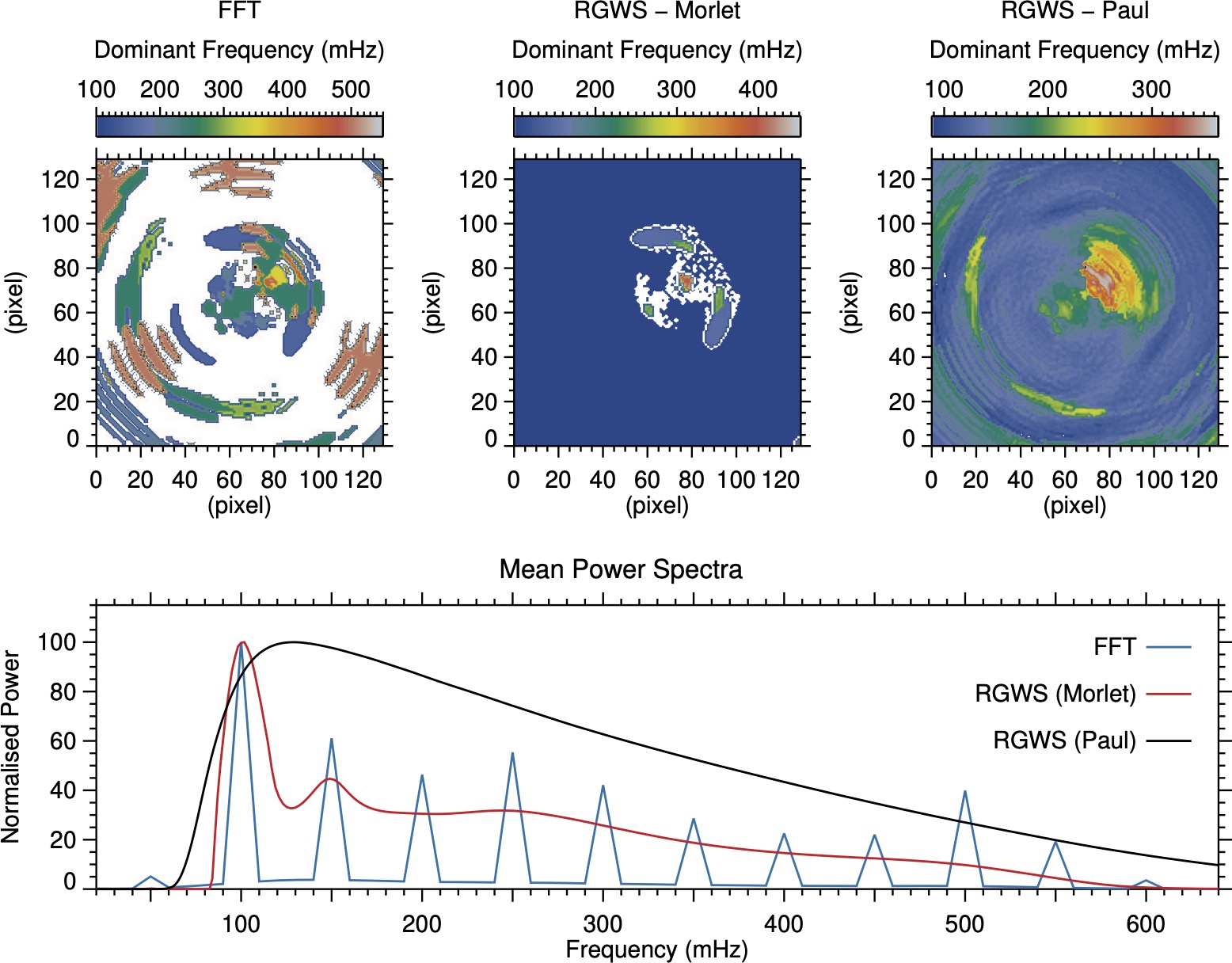
122 | ; pro FIG4__dominant_frequency__mean_spectra
data_dir= 'Synthetic_Data/'
data = readfits(data_dir+'NRMP_signal_3D.fits', /silent)
cadence = 0.5 ; sec
arcsecpx = 1 ; arcsec
nx = n_elements(data[*,0,0])
ny = n_elements(data[0,*,0])
nt = n_elements(data[0,0,*])
time = findgen(nt)*cadence
; ++++++++++++++++++++++++++++++++++++++++++++++++++++++++++++++++++++++++++++++++
colset
device, decomposed=0
; x and y ranges of the image in arcsec
xrg = [ABS(0),ABS(nx-1)]*arcsecpx
yrg = [ABS(0),ABS(ny-1)]*arcsecpx
df = 1000./(time[nt-1]) ; fundamental frequency (frequency resolution) in mHz
; ++++++++++++++++++++++++++++++++++++++++++++++++++++++++++++++++++++++++++++++++
; calculate mean power sepctrum and dominant-frequency map: FFT analysis
;----------------------- plotting
walsa_eps, size=[30,22]
!p.font=0
device,set_font='helvetica'
charsize = 3.0
barthick = 300
distbar = 300
!x.thick=5.0
!y.thick=5.0
line_thick = 4.
!P.Multi = [0, 3, 2]
pos = cgLayout([3,2], OXMargin=[0,0], OYMargin=[0,0], XGap=14, YGap=0)
; To avoid -0 in Dominant Frequency plots!
xy_lables = ['0','20','40','60','80','100','120']
; ppos = pos[*,0]
; xyouts, ppos[0]+((ppos[2]-ppos[0])/2.), ppos[3]+((1-ppos[3])/2.), ALIGNMENT=0.5, CHARSIZE=charsize, /normal, 'Mean Power Spectrum (FFT)', color=cgColor('Black')
; WaLSAtools, /fft, signal=data, time=time, averagedpower=averagedpower, frequencies=frequencies, dominantfreq=dominantfreq, $
; /nosignificance, power=power, rangefreq=rangefreq
;
; save, frequencies, dominantfreq, averagedpower, power, file='save_files/dominant_frequencies_FFT.save'
restore, 'save_files/dominant_frequencies_FFT.save'
walsa_powercolor, 1
walsa_image_plot, dominantfreq, xrange=abs(xrg), yrange=yrg, nobar=0, zrange=round(minmax(dominantfreq,/nan)), $
contour=0, /nocolor, ztitle='FFT!C!CDominant Frequency (mHz)!C', xtitle='(pixel)', ytitle='(pixel)', $
exact=1, aspect=1, cutaspect=1, barpos=1, zlen=-0.45, distbar=barthick, xticklen=-0.04, yticklen=-0.035, $
barthick=barthick, charsize=charsize, position=pos[*,0], resample=2, BARZTICKINTERVAL=100, XTICKNAME=xy_lables, YTICKNAME=xy_lables
cgplot, frequencies, 100*averagedpower/max(averagedpower), yr=[0,115], charsize=charsize, xticklen=-0.045, yticklen=-0.012, position=[0.,0.,1.0,0.345], $
xtitle='Frequency (mHz)', ytitle='Normalised Power', thick=6, Color=cgColor('DodgerBlue'), xr=[20,640], XTICKINTERVAL=50, XTICKNAME=[' ','100',' ','200',' ','300',' ','400',' ','500',' ','600']
xyouts, 310., 126., ALIGNMENT=0.5, CHARSIZE=0.55*charsize, /data, 'Mean Power Spectra', color=cgColor('Black')
;-----------------------------------------------------------------------------
; calculate mean power sepctrum and dominant-frequency map: Wavelet analysis - RGWS Wavelet
; WaLSAtools, /wavelet, /rgws, signal=data, time=time, averagedpower=averagedpower, frequencies=frequencies, dominantfreq=dominantfreq, $
; /nosignificance, power=power, rangefreq=rangefreq, mother='Morlet'
;
; save, frequencies, dominantfreq, averagedpower, power, file='save_files/dominant_frequencies_RGWS_morlet.save'
restore, 'save_files/dominant_frequencies_RGWS_morlet.save'
oplot, frequencies, 100*averagedpower/max(averagedpower), thick=6, Color=cgColor('Red');, /ylog
restore, 'save_files/dominant_frequencies_RGWS_paul.save'
oplot, frequencies, 100*averagedpower/max(averagedpower), thick=6, Color=cgColor('Black');, /ylog
; legends
loc=[600,98] & VSpace=19 & ls = [0,0,0] & colors=['DodgerBlue','Red','Black'] & names = ['FFT','RGWS (Morlet)','RGWS (Paul)']
for fac=0L, 2 do begin
cgPlots, [loc[0],loc[0]+25], [loc[1]-fac*VSpace,loc[1]-fac*VSpace], linestyle=ls[fac], color=cgColor(colors[fac]), thick=6, /data
xyouts, loc[0]-5, loc[1]-fac*VSpace-3.0, names[fac], ALIGNMENT=1, CHARSIZE=charsize/2.0, /data, color=cgColor('Black')
endfor
restore, 'save_files/dominant_frequencies_RGWS_morlet.save'
; ppos = pos[*,0]
; xyouts, ppos[0]+((ppos[2]-ppos[0])/2.), ppos[3]+((1-ppos[3])/2.), ALIGNMENT=0.5, CHARSIZE=charsize, /normal, 'Mean Power Spectrum (Sensible Wavelet)', color=cgColor('Black')
walsa_powercolor, 1
walsa_image_plot, dominantfreq, xrange=xrg, yrange=yrg, nobar=0, zrange=round(minmax(dominantfreq,/nan)), $
contour=0, /nocolor, ztitle='RGWS - Morlet!C!CDominant Frequency (mHz)!C', xtitle='(pixel)', ytitle='(pixel)', $
exact=1, aspect=1, cutaspect=1, barpos=1, zlen=-0.45, distbar=barthick, xticklen=-0.04, yticklen=-0.035, $
barthick=barthick, charsize=charsize, position=pos[*,1], resample=2, BARZTICKINTERVAL=100, XTICKNAME=xy_lables, YTICKNAME=xy_lables
;-----------------------------------------------------------------------------
; calculate mean power sepctrum and dominant-frequency map: Wavelet analysis - RGWS Wavelet
; WaLSAtools, /wavelet, /rgws, signal=data, time=time, averagedpower=averagedpower, frequencies=frequencies, dominantfreq=dominantfreq, $
; /nosignificance, power=power, rangefreq=rangefreq, mother='Paul'
;
; save, frequencies, dominantfreq, averagedpower, power, file='save_files/dominant_frequencies_RGWS_paul.save'
restore, 'save_files/dominant_frequencies_RGWS_paul.save'
; ppos = pos[*,0]
; xyouts, ppos[0]+((ppos[2]-ppos[0])/2.), ppos[3]+((1-ppos[3])/2.), ALIGNMENT=0.5, CHARSIZE=charsize, /normal, 'Mean Power Spectrum (Sensible Wavelet)', color=cgColor('Black')
walsa_powercolor, 1
walsa_image_plot, dominantfreq, xrange=xrg, yrange=yrg, nobar=0, zrange=round(minmax(dominantfreq,/nan)), $
contour=0, /nocolor, ztitle='RGWS - Paul!C!CDominant Frequency (mHz)!C', xtitle='(pixel)', ytitle='(pixel)', $
exact=1, aspect=1, cutaspect=1, barpos=1, zlen=-0.45, distbar=barthick, xticklen=-0.04, yticklen=-0.035, $
barthick=barthick, charsize=charsize, position=pos[*,2], resample=2, BARZTICKINTERVAL=100, XTICKNAME=xy_lables, YTICKNAME=xy_lables
;-----------------------------------------------------------------------------
walsa_endeps, filename='Figures/Fig4_dominant_frequency_mean_power_spectra'
;-----------------------------------------------------------------------------
!P.Multi = 0
Cleanplot, /Silent
stop
end
|