 1
 2
 3
 4
 5
 6
 7
 8
 9
10
11
12
13
14
15
16
17
18
19
20
21
22
23
24
25
26
27
28
29
30
31
32
33
34
35
36
37
38
39
40
41
42
43
44
45
46
47
48
49
50
51
52
53
54
55
56
57
58
59
60
61
62
63
64
65
66
67
68
69
70
71
72
73
74
75
76
77
78
79
80
81
82
83
84
85
86
87
88
89
90
91
92
93
94
95
96
97
98
99
100
101
102
103
104
105
106
107
108
109
110
111
112
113
114
115
116
117
118
119
120
121
122
123
124
125
126
127
128
129
130 | import numpy as np
import matplotlib.pyplot as plt
from matplotlib.ticker import AutoMinorLocator
import matplotlib.gridspec as gridspec
def custom_round(freq):
if freq < 1:
return round(freq, 1)
else:
return round(freq)
# Setting global parameters
plt.rcParams.update({
'font.size': 12, # Global font size
'axes.titlesize': 11, # Title font size
'axes.labelsize': 11, # Axis label font size
'xtick.labelsize': 10, # X-axis tick label font size
'ytick.labelsize': 10, # Y-axis tick label font size
'legend.fontsize': 12, # Legend font size
'figure.titlesize': 12.5, # Figure title font size
'axes.grid': False, # Turn on grid by default
'grid.alpha': 0.5, # Grid transparency
'grid.linestyle': '--', # Grid line style
})
significance_threshold=0.05
plt.rc('axes', linewidth=1.0)
plt.rc('lines', linewidth=1.3)
# Color cycle for consistency across plots
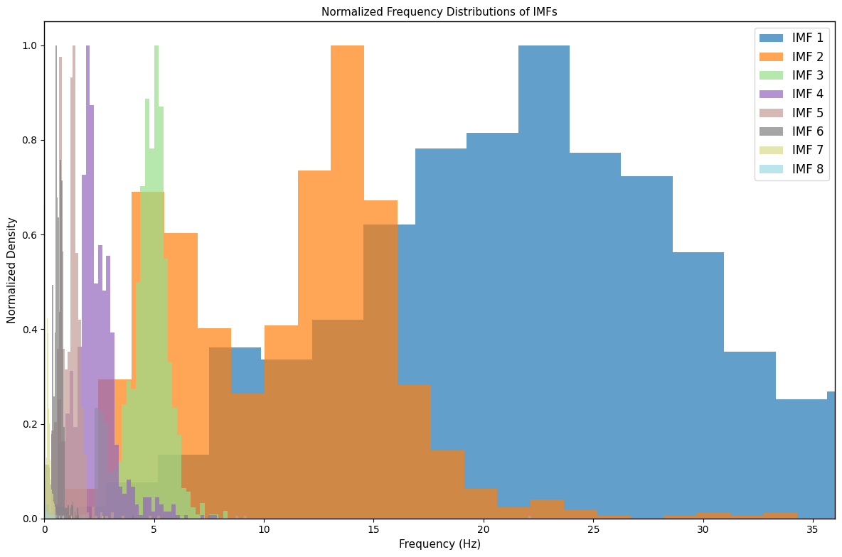
colors = plt.cm.tab10(np.linspace(0, 1, len(imfs)))
# Create a multi-panel plot with custom grid layout
fig = plt.figure(figsize=(8., 9.2), constrained_layout=True)
gs = gridspec.GridSpec(len(imfs) + 2, 2, height_ratios=[1]*len(imfs) + [0.3, 2], figure=fig)
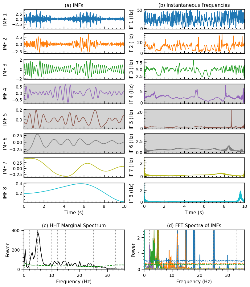
# Plot each IMF and its instantaneous frequency side by side
for i, (imf, freq) in enumerate(zip(imfs, instantaneous_frequencies)):
ax_imf = fig.add_subplot(gs[i, 0])
ax_if = fig.add_subplot(gs[i, 1])
if IMF_significance_levels[i] > significance_threshold:
ax_imf.set_facecolor('lightgray')
ax_imf.plot(time, imf, label=f'IMF {i+1}', color=colors[i])
ax_imf.set_ylabel(f'IMF {i+1}')
ax_imf.yaxis.set_label_coords(-0.16, 0.5) # Align y-axis labels
ax_imf.xaxis.set_minor_locator(AutoMinorLocator(5))
ax_imf.yaxis.set_minor_locator(AutoMinorLocator(3))
ax_imf.tick_params(axis='both', which='major', direction='in', length=6, width=1.0)
ax_imf.tick_params(axis='both', which='minor', direction='in', length=3, width=1.0)
if i < len(imfs) - 1:
ax_imf.set_xticklabels([]) # Hide x labels for all but the last IMF plot
if i == 0:
ax_imf.set_title('(a) IMFs')
ax_imf.tick_params(axis='x', which='both', top=False) # Turn off upper x-axis ticks
ax_imf.set_xlim(0, 10)
if i == len(imfs) - 1:
ax_imf.set_xlabel('Time (s)')
if IMF_significance_levels[i] > significance_threshold:
ax_if.set_facecolor('lightgray')
if len(freq) < len(time):
freq = np.append(freq, freq[-1]) # Extend freq to match the length of time
ax_if.plot(time, freq, label=f'IF {i+1}', color=colors[i])
ax_if.set_ylabel(f'IF {i+1} (Hz)')
ax_if.yaxis.set_label_coords(-0.1, 0.5) # Align y-axis labels
ax_if.xaxis.set_minor_locator(AutoMinorLocator(5))
ax_if.yaxis.set_minor_locator(AutoMinorLocator(5))
ax_if.tick_params(axis='both', which='major', direction='in', length=6, width=1.0)
ax_if.tick_params(axis='both', which='minor', direction='in', length=3, width=1.0)
if i < len(imfs) - 1:
ax_if.set_xticklabels([]) # Hide x labels for all but the last IF plot
if i == 0:
ax_if.set_title('(b) Instantaneous Frequencies')
ax_if.tick_params(axis='x', which='both', top=False) # Turn off upper x-axis ticks
ax_if.set_xlim(0, 10)
if i == len(imfs) - 1:
ax_if.set_xlabel('Time (s)')
# Plot the HHT marginal spectrum and FFT spectra in the last row
# Panel (c): HHT Marginal Spectrum
ax_hht = fig.add_subplot(gs[-1, 0])
# freq_bins = np.linspace(0, 50, len(HHT_power_spectrum)) # Assuming a maximum frequency of 50 Hz for illustration
ax_hht.plot(HHT_freq_bins, HHT_power_spectrum, color='black')
ax_hht.plot(HHT_freq_bins, HHT_significance_level, linestyle='--', color='green')
ax_hht.set_title('(c) HHT Marginal Spectrum')
ax_hht.set_xlabel('Frequency (Hz)')
ax_hht.set_ylabel('Power')
ax_hht.xaxis.set_minor_locator(AutoMinorLocator(5))
ax_hht.yaxis.set_minor_locator(AutoMinorLocator(5))
ax_hht.tick_params(axis='both', which='major', direction='out', length=6, width=1.0)
ax_hht.tick_params(axis='both', which='minor', direction='out', length=3, width=1.0)
ax_hht.tick_params(axis='x', which='both', top=False) # Turn off upper x-axis ticks
ax_hht.set_xlim(0,36)
ax_hht.set_ylim(bottom=0)
# Mark pre-defined frequencies with vertical lines
pre_defined_freq = [2,5,10,12,15,18,25,33]
for freq in pre_defined_freq:
rounded_freq = custom_round(freq)
plt.axvline(x=freq, color='gray', linestyle=':')
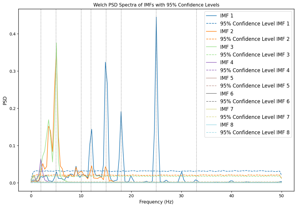
# Panel (d): FFT Spectra of IMFs
ax_fft = fig.add_subplot(gs[-1, 1])
for i, (xf, psd) in enumerate(psd_spectra_fft):
ax_fft.plot(xf, psd, label=f'IMF {i+1}', color=colors[i])
for i, confidence_level in enumerate(confidence_levels_fft):
ax_fft.plot(xf, confidence_level, linestyle='--', color=colors[i])
ax_fft.set_title('(d) FFT Spectra of IMFs')
ax_fft.set_xlabel('Frequency (Hz)')
ax_fft.set_ylabel('Power')
ax_fft.xaxis.set_minor_locator(AutoMinorLocator(5))
ax_fft.yaxis.set_minor_locator(AutoMinorLocator(5))
ax_fft.tick_params(axis='both', which='major', direction='out', length=6, width=1.0)
ax_fft.tick_params(axis='both', which='minor', direction='out', length=3, width=1.0)
ax_fft.tick_params(axis='x', which='both', top=False) # Turn off upper x-axis ticks
ax_fft.set_xlim(0,36)
ax_fft.set_ylim(0,2.5)
# Mark pre-defined frequencies with vertical lines
pre_defined_freq = [2,5,10,12,15,18,25,33]
for freq in pre_defined_freq:
rounded_freq = custom_round(freq)
plt.axvline(x=freq, color='gray', linestyle=':')
# Save the figure as a PDF
pdf_path = 'Figures/FigS2_EMD_analysis.pdf'
WaLSA_save_pdf(fig, pdf_path, color_mode='CMYK', dpi=300, bbox_inches='tight', pad_inches=0)
plt.show()
|