Figures that are newly created, modified, or unrelated to the published article may be used under the terms of the Apache License.
Disclaimer: This notebook and its code are provided "as is", without warranty of any kind, express or implied. Refer to the license for more details.
1 2 3 4 5 6 7 8 910111213
importnumpyasnpfromastropy.ioimportfitsfromWaLSAtoolsimportWaLSAtools,WaLSA_save_pdf# Load FITS datadata_dir='Synthetic_Data/'hdul=fits.open(data_dir+'NRMP_signal_3D.fits')signal_3d=hdul[0].data# 3D synthetic datatime=hdul[1].data# Time array, saved in the second HDU (Extension HDU 1)hdul.close()# Computed POD modes using WaLSAtoolspod_results=WaLSAtools(signal=signal_3d,time=time,method='pod',num_modes=10)
Starting POD analysis ....
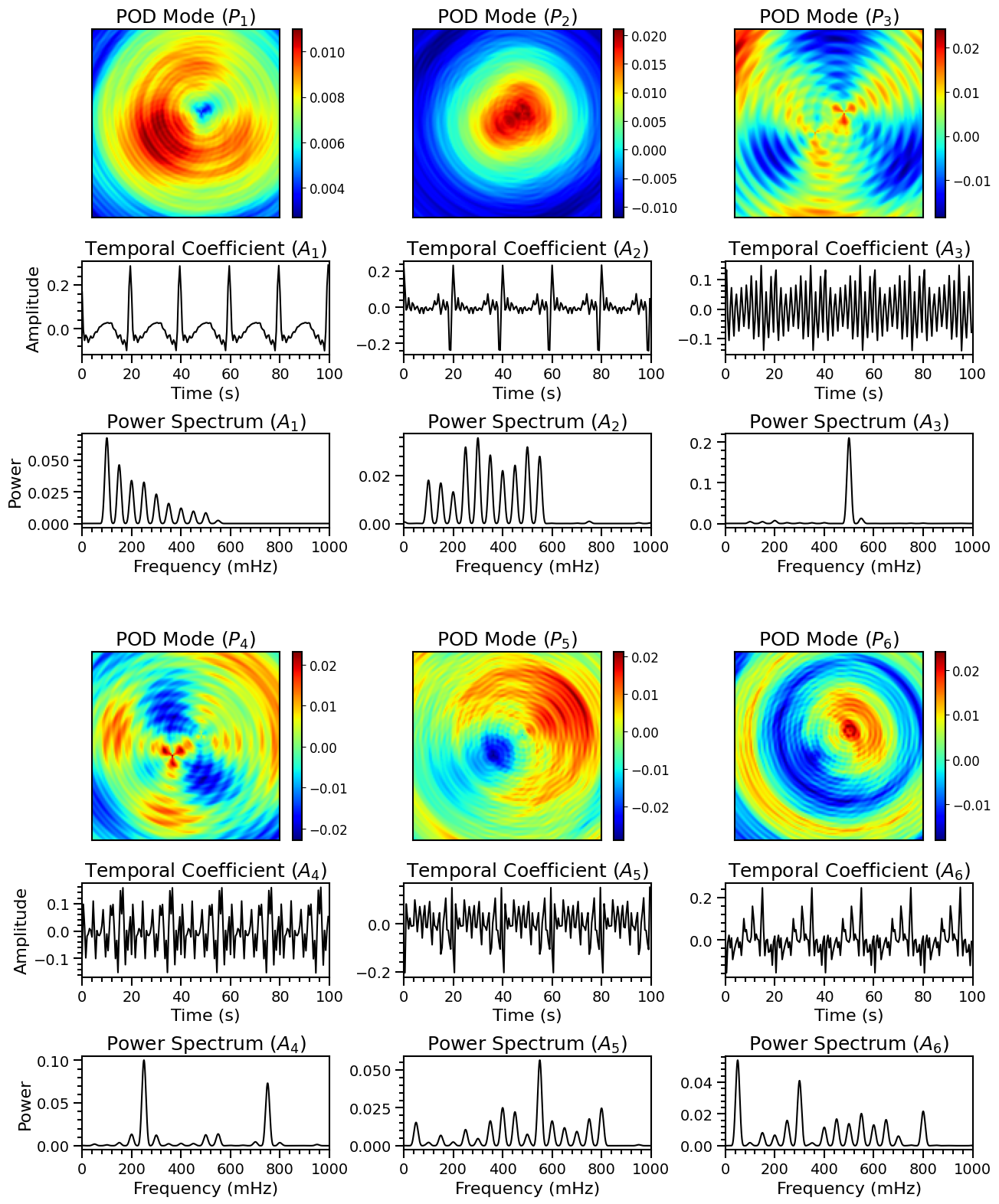
Processing a 3D cube with shape (200, 130, 130).
POD analysis completed.
Top 10 frequencies and normalized power values:
[[0.1, 1.0], [0.15, 0.7], [0.25, 0.61], [0.2, 0.54], [0.3, 0.47], [0.5, 0.39], [0.35, 0.32], [0.4, 0.25], [0.45, 0.24], [0.55, 0.18]]
Total variance contribution of the first 10 modes: 96.01%
---- POD/SPOD Results Summary ----
input_data (ndarray, Shape: (200, 130, 130)): Original input data, mean subtracted (Shape: (Nt, Ny, Nx))
spatial_mode (ndarray, Shape: (200, 130, 130)): Reshaped spatial modes matching the dimensions of the input data (Shape: (Nmodes, Ny, Nx))
temporal_coefficient (ndarray, Shape: (200, 200)): Temporal coefficients associated with each spatial mode (Shape: (Nmodes, Nt))
eigenvalue (ndarray, Shape: (200,)): Eigenvalues corresponding to singular values squared (Shape: (Nmodes))
eigenvalue_contribution (ndarray, Shape: (200,)): Eigenvalue contribution of each mode (Shape: (Nmodes))
cumulative_eigenvalues (list, Shape: (10,)): Cumulative percentage of eigenvalues for the first "num_cumulative_modes" modes (Shape: (num_cumulative_modes))
combined_welch_psd (ndarray, Shape: (8193,)): Combined Welch power spectral density for the temporal coefficients of the firts "num_modes" modes (Shape: (Nf))
frequencies (ndarray, Shape: (8193,)): Frequencies identified in the Welch spectrum (Shape: (Nf))
combined_welch_significance (ndarray, Shape: (8193,)): Significance threshold of the combined Welch spectrum (Shape: (Nf,))
reconstructed (ndarray, Shape: (130, 130)): Reconstructed frame at the specified timestep using the top "num_modes" modes (Shape: (Ny, Nx))
sorted_frequencies (ndarray, Shape: (21,)): Frequencies identified in the Welch combined power spectrum (Shape: (Nfrequencies))
frequency_filtered_modes (ndarray, Shape: (200, 130, 130, 10)): Frequency-filtered spatial POD modes for the first "num_top_frequencies" frequencies (Shape: (Nt, Ny, Nx, num_top_frequencies))
frequency_filtered_modes_frequencies (ndarray, Shape: (10,)): Frequencies corresponding to the frequency-filtered modes (Shape: (num_top_frequencies))
SPOD_spatial_modes (NoneType, Shape: None): SPOD spatial modes if SPOD is used (Shape: (Nspod_modes, Ny, Nx))
SPOD_temporal_coefficients (NoneType, Shape: None): SPOD temporal coefficients if SPOD is used (Shape: (Nspod_modes, Nt))
p (ndarray, Shape: (16900, 200)): Left singular vectors (spatial modes) from SVD (Shape: (Nx, Nmodes))
s (ndarray, Shape: (200,)): Singular values from SVD (Shape: (Nmodes))
a (ndarray, Shape: (200, 200)): Right singular vectors (temporal coefficients) from SVD (Shape: (Nmodes, Nt))
importmatplotlib.pyplotaspltimportmatplotlib.gridspecasgridspecfrommatplotlib.tickerimportAutoMinorLocatorfromscipy.signalimportwelch# Setting global parametersplt.rcParams.update({'font.size':14,# Global font size'axes.titlesize':18,# Title font size'axes.labelsize':16,# Axis label font size'xtick.labelsize':12,# X-axis tick label font size'ytick.labelsize':12,# Y-axis tick label font size'legend.fontsize':14,# Legend font size'figure.titlesize':20,# Figure title font size'axes.grid':False,# Turn off grid by default'grid.alpha':0.5,# Grid transparency'grid.linestyle':'--',# Grid line style})fig=plt.figure(figsize=(15,19))# Create a figure with specified size# Create subplots with GridSpecgs1=gridspec.GridSpec(9,3,height_ratios=[1,0.5,-0.04,0.5,0.2,1,0.5,-0.04,0.5],figure=fig,hspace=0.5,wspace=0.3)# Plot each column of p as an image in a subplotforminrange(3):# First set of 3 modesax_img=plt.subplot(gs1[0,m])ax_img.set_title(f'POD Mode ($P_{m+1}$)')img=ax_img.imshow(spatial_modes[m,:,:],cmap='jet',aspect='equal',origin='lower')colorbar=plt.colorbar(img,ax=ax_img,orientation='vertical',shrink=1.0)colorbar.outline.set_linewidth(1.5)ax_img.set_xticks([])# Remove x ticksax_img.set_yticks([])# Remove y ticksforspineinax_img.spines.values():spine.set_linewidth(1.5)ax_line=plt.subplot(gs1[1,m])ax_line.plot(time,temporal_coefficients[m,:],'k')ax_line.set_title(f'Temporal Coefficient ($A_{m+1}$)')ax_line.set_xlabel('Time (s)')# X labelifm==0:ax_line.set_ylabel('Amplitude')# Y labelax_line.tick_params(axis='y',labelsize=8)# Adjust y tick label sizeax_line.grid(False)# Turn off gridax_line.xaxis.set_minor_locator(AutoMinorLocator(5))ax_line.yaxis.set_minor_locator(AutoMinorLocator(5))ax_line.tick_params(axis='both',which='major',direction='out',length=8,width=1.5)ax_line.tick_params(axis='both',which='minor',direction='out',length=4,width=1.5)ax_line.tick_params(axis='both',labelsize=14)forspineinax_line.spines.values():spine.set_linewidth(1.5)ax_line.set_xlim(0,100)ax_welch=plt.subplot(gs1[3,m])f,px=welch(temporal_coefficients[m,:]-np.mean(temporal_coefficients[m,:]),nperseg=150,noverlap=25,nfft=2**14,fs=2)ax_welch.plot(f*1000.,px,'k')ax_welch.set_title(f'Power Spectrum ($A_{m+1}$)')ax_welch.set_xlabel('Frequency (mHz)')# X labelifm==0:ax_welch.set_ylabel('Power')# Y labelax_welch.tick_params(axis='y',labelsize=8)# Adjust y tick label sizeax_welch.grid(False)# Turn off gridax_welch.xaxis.set_minor_locator(AutoMinorLocator(5))ax_welch.yaxis.set_minor_locator(AutoMinorLocator(5))ax_welch.tick_params(axis='both',which='major',direction='out',length=8,width=1.5)ax_welch.tick_params(axis='both',which='minor',direction='out',length=4,width=1.5)ax_welch.tick_params(axis='both',labelsize=14)forspineinax_welch.spines.values():spine.set_linewidth(1.5)ax_welch.set_xlim(0,1000)# Create a separate GridSpec for the spacing between the two setsgs_space=gridspec.GridSpec(1,1,top=0.98,bottom=0.95,hspace=0.5,wspace=0.5,figure=fig)forminrange(3,6):# Second set of 3 modesrow=m-3col=m%3ax_img=plt.subplot(gs1[5,col])ax_img.set_title(f'POD Mode ($P_{m+1}$)')img=ax_img.imshow(spatial_modes[m,:,:],cmap='jet',aspect='equal',origin='lower')colorbar=plt.colorbar(img,ax=ax_img,orientation='vertical',shrink=1.0)colorbar.outline.set_linewidth(1.5)ax_img.set_xticks([])# Remove x ticksax_img.set_yticks([])# Remove y ticksforspineinax_img.spines.values():spine.set_linewidth(1.5)ax_line=plt.subplot(gs1[6,col])ax_line.plot(time,temporal_coefficients[m,:],'k')ax_line.set_title(f'Temporal Coefficient ($A_{m+1}$)')ax_line.set_xlabel('Time (s)')# X labelifm==3:ax_line.set_ylabel('Amplitude')# Y labelax_line.tick_params(axis='y',labelsize=8)# Adjust y tick label sizeax_line.grid(False)# Turn off gridax_line.xaxis.set_minor_locator(AutoMinorLocator(5))ax_line.yaxis.set_minor_locator(AutoMinorLocator(5))ax_line.tick_params(axis='both',which='major',direction='out',length=8,width=1.5)ax_line.tick_params(axis='both',which='minor',direction='out',length=4,width=1.5)ax_line.tick_params(axis='both',labelsize=14)forspineinax_line.spines.values():spine.set_linewidth(1.5)ax_line.set_xlim(0,100)ax_welch=plt.subplot(gs1[8,col])f,px=welch(temporal_coefficients[m,:]-np.mean(temporal_coefficients[m,:]),nperseg=150,noverlap=25,nfft=2**14,fs=2)ax_welch.plot(f*1000.,px,'k')ax_welch.set_title(f'Power Spectrum ($A_{m+1}$)')ax_welch.set_xlabel('Frequency (mHz)')# X labelifm==3:ax_welch.set_ylabel('Power')# Y labelax_welch.tick_params(axis='y',labelsize=8)# Adjust y tick label sizeax_welch.grid(False)# Turn off gridax_welch.xaxis.set_minor_locator(AutoMinorLocator(5))ax_welch.yaxis.set_minor_locator(AutoMinorLocator(5))ax_welch.tick_params(axis='both',which='major',direction='out',length=8,width=1.5)ax_welch.tick_params(axis='both',which='minor',direction='out',length=4,width=1.5)ax_welch.tick_params(axis='both',labelsize=14)forspineinax_welch.spines.values():spine.set_linewidth(1.5)ax_welch.set_xlim(0,1000)# Save the figure as a PDFpdf_path='Figures/FigS5_POD_analysis.pdf'WaLSA_save_pdf(fig,pdf_path,color_mode='CMYK',dpi=300,bbox_inches='tight',pad_inches=0)# Show the plotplt.show()
GPL Ghostscript 10.04.0 (2024-09-18)
Copyright (C) 2024 Artifex Software, Inc. All rights reserved.
This software is supplied under the GNU AGPLv3 and comes with NO WARRANTY:
see the file COPYING for details.
Processing pages 1 through 1.
Page 1
PDF saved in CMYK format as 'Figures/FigS5_POD_analysis.pdf'