Figures that are newly created, modified, or unrelated to the published article may be used under the terms of the Apache License.
Disclaimer: This notebook and its code are provided "as is", without warranty of any kind, express or implied. Refer to the license for more details.
1 2 3 4 5 6 7 8 9101112131415161718192021
fromastropy.ioimportfitsfromWaLSAtoolsimportWaLSAtools,WaLSA_save_pdf# Load FITS datadata_dir='Synthetic_Data/'hdul=fits.open(data_dir+'NRMP_signal_3D.fits')signal_3d=hdul[0].data# 3D synthetic datatime=hdul[1].data# Time array, saved in the second HDU (Extension HDU 1)hdul.close()# Computed POD modes using WaLSAtoolspod_results=WaLSAtools(signal=signal_3d,time=time,method='pod',num_modes=10,num_top_frequencies=10,num_cumulative_modes=50,timestep_to_reconstruct=1,num_modes_reconstruct=22)
Starting POD analysis ....
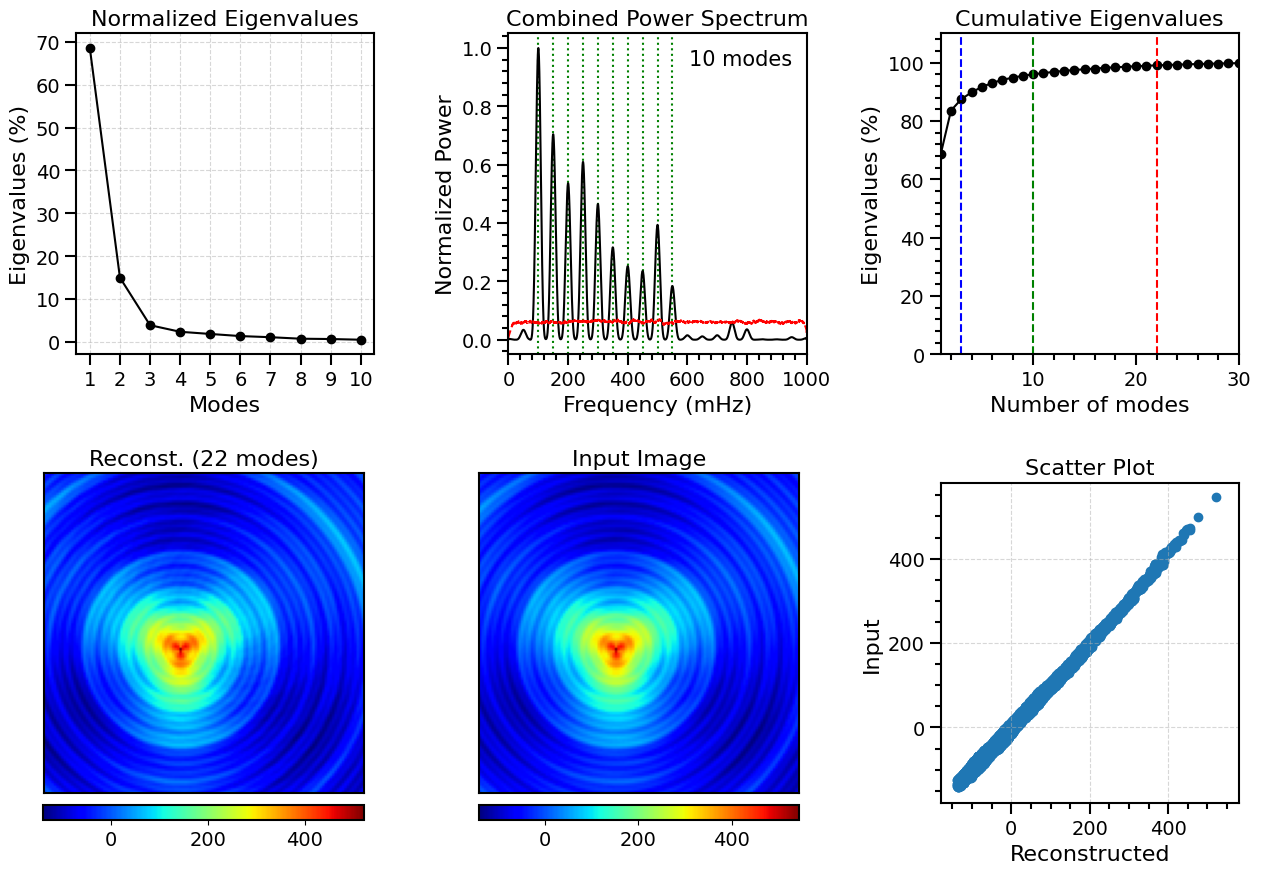
Processing a 3D cube with shape (200, 130, 130).
POD analysis completed.
Top 10 frequencies and normalized power values:
[[0.1, 1.0], [0.15, 0.7], [0.25, 0.61], [0.2, 0.54], [0.3, 0.47], [0.5, 0.39], [0.35, 0.32], [0.4, 0.25], [0.45, 0.24], [0.55, 0.18]]
Total variance contribution of the first 10 modes: 96.01%
---- POD/SPOD Results Summary ----
input_data (ndarray, Shape: (200, 130, 130)): Original input data, mean subtracted (Shape: (Nt, Ny, Nx))
spatial_mode (ndarray, Shape: (200, 130, 130)): Reshaped spatial modes matching the dimensions of the input data (Shape: (Nmodes, Ny, Nx))
temporal_coefficient (ndarray, Shape: (200, 200)): Temporal coefficients associated with each spatial mode (Shape: (Nmodes, Nt))
eigenvalue (ndarray, Shape: (200,)): Eigenvalues corresponding to singular values squared (Shape: (Nmodes))
eigenvalue_contribution (ndarray, Shape: (200,)): Eigenvalue contribution of each mode (Shape: (Nmodes))
cumulative_eigenvalues (list, Shape: (50,)): Cumulative percentage of eigenvalues for the first "num_cumulative_modes" modes (Shape: (num_cumulative_modes))
combined_welch_psd (ndarray, Shape: (8193,)): Combined Welch power spectral density for the temporal coefficients of the firts "num_modes" modes (Shape: (Nf))
frequencies (ndarray, Shape: (8193,)): Frequencies identified in the Welch spectrum (Shape: (Nf))
combined_welch_significance (ndarray, Shape: (8193,)): Significance threshold of the combined Welch spectrum (Shape: (Nf,))
reconstructed (ndarray, Shape: (130, 130)): Reconstructed frame at the specified timestep using the top "num_modes" modes (Shape: (Ny, Nx))
sorted_frequencies (ndarray, Shape: (21,)): Frequencies identified in the Welch combined power spectrum (Shape: (Nfrequencies))
frequency_filtered_modes (ndarray, Shape: (200, 130, 130, 10)): Frequency-filtered spatial POD modes for the first "num_top_frequencies" frequencies (Shape: (Nt, Ny, Nx, num_top_frequencies))
frequency_filtered_modes_frequencies (ndarray, Shape: (10,)): Frequencies corresponding to the frequency-filtered modes (Shape: (num_top_frequencies))
SPOD_spatial_modes (NoneType, Shape: None): SPOD spatial modes if SPOD is used (Shape: (Nspod_modes, Ny, Nx))
SPOD_temporal_coefficients (NoneType, Shape: None): SPOD temporal coefficients if SPOD is used (Shape: (Nspod_modes, Nt))
p (ndarray, Shape: (16900, 200)): Left singular vectors (spatial modes) from SVD (Shape: (Nx, Nmodes))
s (ndarray, Shape: (200,)): Singular values from SVD (Shape: (Nmodes))
a (ndarray, Shape: (200, 200)): Right singular vectors (temporal coefficients) from SVD (Shape: (Nmodes, Nt))
importnumpyasnpimportmatplotlib.pyplotaspltimportmatplotlib.gridspecasgridspecfrommatplotlib.tickerimportAutoMinorLocatorimportmatplotlib.tickerastickerfrommatplotlib.tickerimportMaxNLocator# Setting global parameters for the plotsplt.rcParams.update({'font.size':14,# Global font size'axes.titlesize':16,# Title font size'axes.labelsize':16,# Axis label font size'xtick.labelsize':14,# X-axis tick label font size'ytick.labelsize':14,# Y-axis tick label font size'legend.fontsize':14,# Legend font size'figure.titlesize':17,# Figure title font size'axes.grid':False,# Turn off grid by default'grid.alpha':0.5,# Grid transparency'grid.linestyle':'--',# Grid line style})fig=plt.figure(figsize=(15,10))# Create subplots with GridSpecgs1=gridspec.GridSpec(2,3,figure=fig,wspace=0.45,hspace=0.4)# Plot normalized eigenvaluesax_ev=plt.subplot(gs1[0,0])ax_ev.set_title(f'Normalized Eigenvalues')mode_nums=np.arange(1,11)ax_ev.plot(mode_nums,100*eigenvalue_contribution[0:10],'k-o')ax_ev.set_xlabel('Modes')ax_ev.set_ylabel('Eigenvalues (%)')ax_ev.grid(True)ax_ev.xaxis.set_major_locator(ticker.MultipleLocator(1))ax_ev.tick_params(axis='both',which='major',direction='out',length=8,width=1.5)ax_ev.tick_params(axis='both',labelsize=14)forspineinax_ev.spines.values():spine.set_linewidth(1.5)# Plot combined power spectrumax_freq=plt.subplot(gs1[0,1])pre_defined_freq=[100,150,200,250,300,350,400,450,500,550]forfreqinpre_defined_freq:ax_freq.axvline(x=freq,color='green',linestyle=':',linewidth=1.5)ax_freq.plot(frequencies*1000.,combined_welch_psd/np.max(combined_welch_psd),'k')ax_freq.plot(frequencies*1000.,combined_welch_significance,'r--',label='95% Significance Threshold')ax_freq.set_title(f'Combined Power Spectrum')ax_freq.set_xlabel('Frequency (mHz)')ax_freq.set_ylabel('Normalized Power')ax_freq.grid(False)ax_freq.xaxis.set_minor_locator(AutoMinorLocator(5))ax_freq.yaxis.set_minor_locator(AutoMinorLocator(5))ax_freq.tick_params(axis='both',which='major',direction='out',length=8,width=1.5)ax_freq.tick_params(axis='both',which='minor',direction='out',length=4,width=1.5)ax_freq.tick_params(axis='both',labelsize=14)forspineinax_freq.spines.values():spine.set_linewidth(1.5)ax_freq.set_xlim(0,1000)ax_freq.text(0.95,0.95,'10 modes',transform=ax_freq.transAxes,fontsize=15,verticalalignment='top',horizontalalignment='right')# Plot cumulative eigenvaluesax_freq=plt.subplot(gs1[0,2])ax_freq.plot(cumulative_eigenvalues,'k-o')ax_freq.set_title(f'Cumulative Eigenvalues')ax_freq.set_xlabel('Number of modes')ax_freq.set_ylabel('Eigenvalues (%)')ax_freq.grid(False)ax_freq.xaxis.set_minor_locator(AutoMinorLocator(5))ax_freq.yaxis.set_minor_locator(AutoMinorLocator(5))ax_freq.tick_params(axis='both',which='major',direction='out',length=8,width=1.5)ax_freq.tick_params(axis='both',which='minor',direction='out',length=4,width=1.5)ax_freq.tick_params(axis='both',labelsize=14)forspineinax_freq.spines.values():spine.set_linewidth(1.5)ax_freq.set_xlim(1,30)ax_freq.set_ylim(0,110)# Identify indices where 90% and 95% is reachedthresholds=[84,96,99]colors=['blue','green','red']forthreshold,colorinzip(thresholds,colors):index=next(ifori,vinenumerate(cumulative_eigenvalues)ifv>=threshold)ax_freq.axvline(x=index,color=color,linestyle='--',label=f'{threshold}% at mode {index}')# Plot reconstructed image for frame number 1 (using the first 22 modes)im_recon=plt.subplot(gs1[1,0])im_recon.set_title('Reconst. (22 modes)')img=im_recon.imshow(reconstructed,cmap='jet',aspect='equal',origin='lower')im_recon.set_xticks([])# Remove x ticksim_recon.set_yticks([])# Remove y ticksforspineinim_recon.spines.values():spine.set_linewidth(1.5)im_recon.set_position([0.05,0.12,0.32,0.32])# Adjust these values (left, bottom, width, height)# Create a new axis for the colorbar and set its positioncax=fig.add_axes([0.103,0.093,0.2135,0.015])# Adjust these values (left, bottom, width, height)colorbar=plt.colorbar(img,cax=cax,orientation='horizontal')colorbar.outline.set_linewidth(1.5)# Plot input image (mean subtracted) for frame number 1 im_input=plt.subplot(gs1[1,1])im_input.set_title('Input Image')img2=im_input.imshow(input_data[1,:,:],cmap='jet',aspect='equal',origin='lower')im_input.set_xticks([])# Remove x ticksim_input.set_yticks([])# Remove y ticksforspineinim_input.spines.values():spine.set_linewidth(1.5)im_input.set_position([0.34,0.12,0.32,0.32])# Adjust these values (left, bottom, width, height)# Create a new axis for the colorbar and set its positioncax2=fig.add_axes([0.3935,0.093,0.2135,0.015])# Adjust these values (left, bottom, width, height)colorbar=plt.colorbar(img2,cax=cax2,orientation='horizontal')colorbar.outline.set_linewidth(1.5)# Add scatter plotax_scatter=plt.subplot(gs1[1,2])ax_scatter.set_title('Scatter Plot')ax_scatter.scatter(reconstructed,input_data[1,:,:])ax_scatter.set_xlabel('Reconstructed')ax_scatter.set_ylabel('Input')ax_scatter.grid(True)ax_scatter.xaxis.set_minor_locator(AutoMinorLocator(4))ax_scatter.yaxis.set_minor_locator(AutoMinorLocator(4))ax_scatter.xaxis.set_major_locator(MaxNLocator(nbins=4))ax_scatter.yaxis.set_major_locator(MaxNLocator(nbins=4))ax_scatter.tick_params(axis='both',which='major',direction='out',length=8,width=1.5)ax_scatter.tick_params(axis='both',which='minor',direction='out',length=4,width=1.5)ax_scatter.tick_params(axis='both',labelsize=14)forspineinax_scatter.spines.values():spine.set_linewidth(1.5)ax_scatter.set_xlim(-180,580)ax_scatter.set_ylim(-180,580)# Save the figure as a PDFpdf_path='Figures/FigS6_POD_eigenvalues_powerspectrum.pdf'WaLSA_save_pdf(fig,pdf_path,color_mode='CMYK',dpi=300,bbox_inches='tight',pad_inches=0)plt.show()
GPL Ghostscript 10.04.0 (2024-09-18)
Copyright (C) 2024 Artifex Software, Inc. All rights reserved.
This software is supplied under the GNU AGPLv3 and comes with NO WARRANTY:
see the file COPYING for details.
Processing pages 1 through 1.
Page 1
PDF saved in CMYK format as 'Figures/FigS6_POD_egenvalues_powerspectrum.pdf'