Worked Example - NRMP: Empirical Mode Decomposition (EMD)
This example demonstrates the application of Empirical Mode Decomposition (EMD) to a synthetic 1D signal. EMD is a data-driven technique that decomposes a signal into a set of Intrinsic Mode Functions (IMFs), each representing a distinct oscillatory mode with its own time-varying amplitude and frequency.
Analysis and Figure
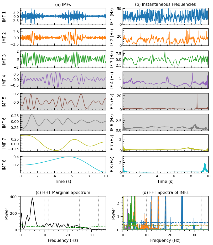
The figure below shows the results of applying EMD to the synthetic 1D signal.
Methods used:
- Empirical Mode Decomposition (EMD)
- Hilbert Transform (to calculate instantaneous frequencies)
- Fast Fourier Transform (FFT) (to analyze the frequency content of the IMFs)
WaLSAtools version: 1.0
These particular analyses generate the figure below (Supplementary Figure S2 in Nature Reviews Methods Primers; copyrighted). For a full description of the datasets and the analyses performed, see the associated article. See the source code at the bottom of this page (or here on Github) for a complete analyses and the plotting routines used to generate this figure.
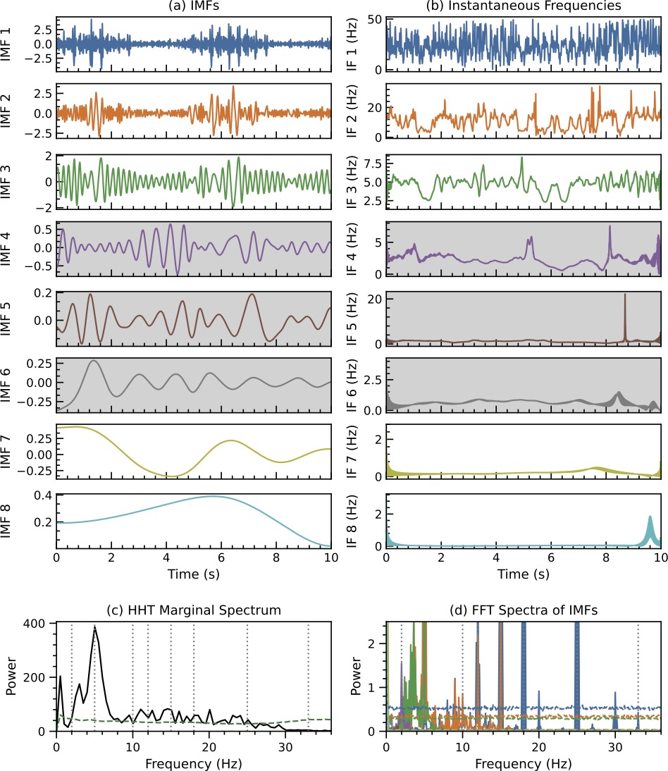
Figure Caption: EMD analysis of the synthetic 1D signal. (a) IMFs extracted from the synthetic signal using EMD. IMFs 4, 5, and 6 are marked with the grey background as non-significant (at 5%) based on a significance test. (b) Instantaneous frequencies of each IMF. © HHT marginal spectrum. (d) FFT power spectra of individual IMFs. The dashed lines in both panels © and (d) indicate the 95% confidence levels. Note that the powers in panels © and (d) are shown in arbitrary units. The dotted vertical lines mark the oscillation frequencies of the synthetic signal.
Source code
© 2025 WaLSA Team - Shahin Jafarzadeh et al.
This notebook is part of the WaLSAtools package (v1.0), provided under the Apache License, Version 2.0.
You may use, modify, and distribute this notebook and its contents under the terms of the license.
Important Note on Figures: Figures generated using this notebook that are identical to or derivative of those published in:
Jafarzadeh, S., Jess, D. B., Stangalini, M. et al. 2025, Nature Reviews Methods Primers, 5, 21
are copyrighted by Nature Reviews Methods Primers. Any reuse of such figures requires explicit permission from the journal.
Free access to a view-only version: https://WaLSA.tools/nrmp
Supplementary Information: https://WaLSA.tools/nrmp-si
Figures that are newly created, modified, or unrelated to the published article may be used under the terms of the Apache License.
Disclaimer: This notebook and its code are provided "as is", without warranty of any kind, express or implied. Refer to the license for more details.
1 2 3 4 5 6 7 8 9 10 11 12 13 14 15 16 17 18 19 20 | |
Detrending and apodization complete.
EMD processed.
1 2 3 4 5 6 7 8 9 10 11 12 13 14 15 16 17 18 19 20 21 22 23 24 25 26 27 28 29 30 31 32 33 34 35 36 37 38 39 40 41 42 43 44 45 46 47 48 49 50 51 52 53 54 55 56 57 58 59 60 61 62 63 64 65 66 67 68 69 70 71 72 73 74 75 76 77 78 79 80 81 82 83 84 85 86 87 88 89 90 91 92 93 94 95 96 97 98 99 100 101 102 103 104 105 106 107 108 109 110 111 112 113 114 115 116 117 118 119 120 121 122 123 124 125 126 127 128 129 130 | |
GPL Ghostscript 10.04.0 (2024-09-18)
Copyright (C) 2024 Artifex Software, Inc. All rights reserved.
This software is supplied under the GNU AGPLv3 and comes with NO WARRANTY:
see the file COPYING for details.
Processing pages 1 through 1.
Page 1
PDF saved in CMYK format as 'Figures/FigS2_EMD_analysis.pdf'
1 2 3 4 5 6 7 8 9 10 11 12 13 14 15 16 17 18 | |
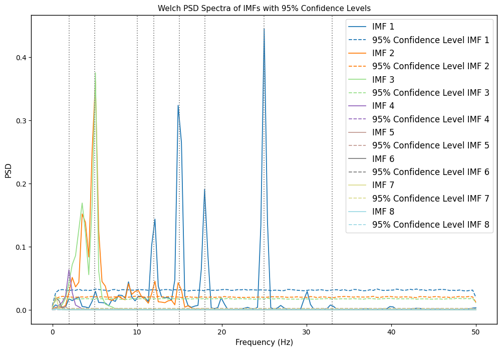
# Further tests
# EMD & HHT Calculations using WaLSAtools - Welch PSD Spectra
_, _, _, psd_spectra_welch, confidence_levels_welch, _, _, _ = WaLSAtools(
    signal = signal,
    time = time,
    method = 'emd',
    siglevel = 0.95,
    Welch_psd = True
)

plt.figure(figsize=(12, 8))
colors = plt.cm.tab20(np.linspace(0, 1, len(psd_spectra_welch)))

for i, (f, psd) in enumerate(psd_spectra_welch):
    plt.plot(f, psd, color=colors[i], label=f'IMF {i + 1}')
    plt.plot(f, confidence_levels_welch[i], color=colors[i], linestyle='--', label=f'95% Confidence Level IMF {i + 1}')

# Mark pre-defined frequencies with vertical lines
pre_defined_freq = [2,5,10,12,15,18,25,33]
for freq in pre_defined_freq:
    plt.axvline(x=freq, color='gray', linestyle=':')

plt.xlabel('Frequency (Hz)')
plt.ylabel('PSD')
plt.title('Welch PSD Spectra of IMFs with 95% Confidence Levels')
plt.legend()
plt.show()
Detrending and apodization complete.
EMD processed.