Skip to content

Worked Example - NRMP: k-ω and POD Analysis

This example demonstrates the application of k-ω filtering and Proper Orthogonal Decomposition (POD) to a synthetic spatio-temporal dataset. The dataset consists of a time series of 2D images, representing the evolution of wave patterns over both space and time. By analysing this dataset with k-ω and POD, we can identify and isolate specific wave modes, revealing their spatial structures and temporal dynamics.

k-ω Analysis

k-ω analysis is a technique used to study wave phenomena in spatio-temporal datasets. It involves calculating the power spectrum of the data in both the spatial domain (wavenumber, k) and the temporal domain (frequency, ω). The resulting k-ω diagram shows how wave power is distributed across different spatial and temporal scales, providing insights into wave dispersion relations and the characteristics of different wave modes.

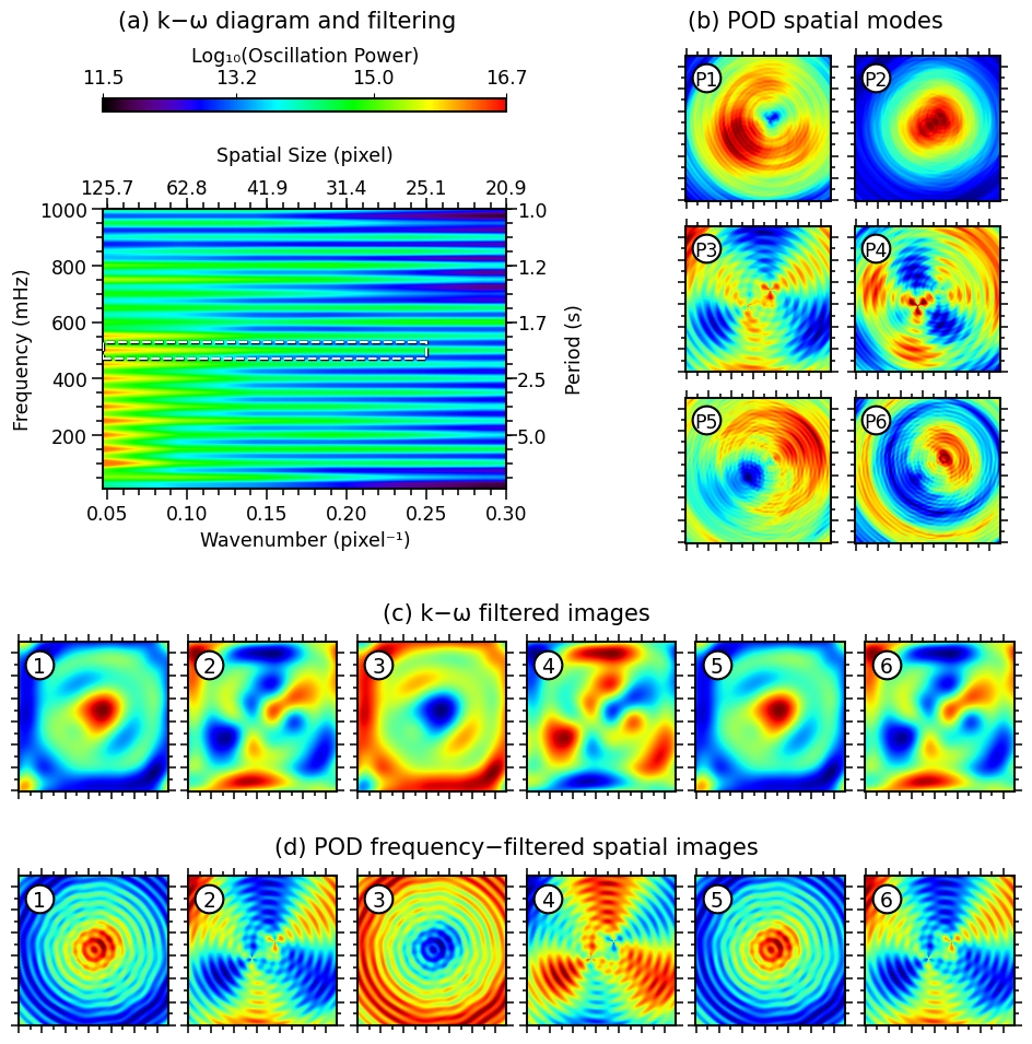
In this example, we apply k-ω analysis to the synthetic spatio-temporal dataset to identify and isolate a specific wave mode with a frequency of 500 mHz and wavenumbers between 0.05 and 0.25 pixel-1. We then use Fourier filtering to extract this wave mode from the dataset, revealing its spatial structure and temporal evolution.

Proper Orthogonal Decomposition (POD)

Proper Orthogonal Decomposition (POD) is a powerful technique for analysing multi-dimensional data. It identifies dominant spatial patterns, or modes, that capture the most significant variations in the data. POD is particularly useful for reducing the dimensionality of complex datasets and extracting coherent structures.

In this example, we apply POD to the synthetic spatio-temporal dataset to identify the dominant spatial modes of oscillation. We then apply frequency filtering to the temporal coefficients of these modes to isolate the 500 mHz wave mode. This allows us to compare the results of k-ω filtering and POD-based filtering, highlighting their respective strengths and limitations.

Analysis and Figure

The figure below shows a comparison of k-ω filtering and POD analysis applied to the synthetic spatio-temporal dataset.

Methods used:

  • k-ω analysis with Fourier filtering
  • Proper Orthogonal Decomposition (POD) with frequency filtering

WaLSAtools version: 1.0

These particular analyses generate the figure below (Figure 5 in Nature Reviews Methods Primers; copyrighted). For a full description of the datasets and the analyses performed, see the associated article. See the source code at the bottom of this page (or here on Github) for a complete analyses and the plotting routines used to generate this figure.

jpg

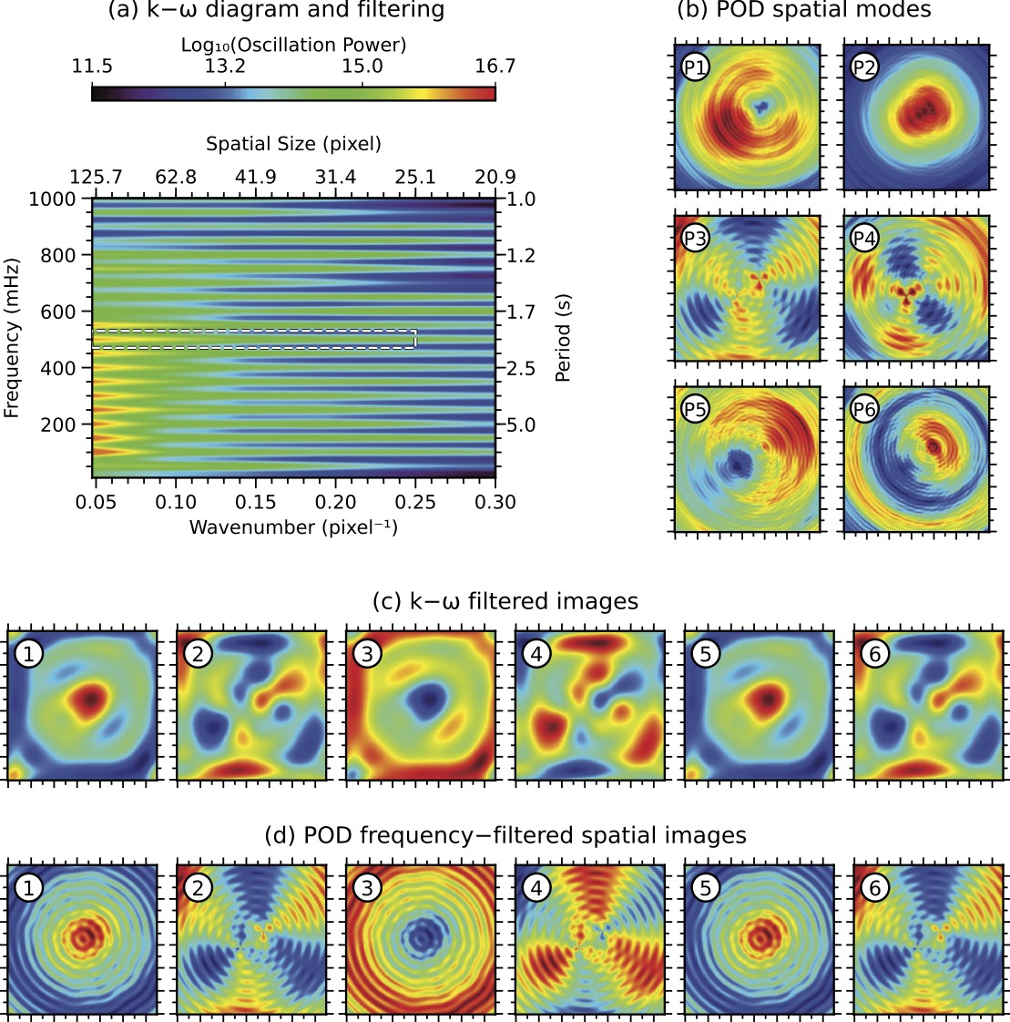
Figure Caption: Comparison of k-ω filtering and POD analysis. (a) k-ω power diagram of the synthetic spatio-temporal dataset with a targeted filtering region (dashed lines). (b) First six spatial modes from POD analysis (each 130×130 pixels2). © First six frames of the k-ω filtered datacube centred at 500 mHz (±30 mHz) and wavenumbers 0.05−0.25 pixel-1. (d) First six frames of the frequency-filtered POD reconstruction at 500 mHz using the first 22 POD modes (99% of total variance). All images and spatial modes are plotted with their own minimum and maximum values to highlight detailed structures within them.

Source code

© 2025 WaLSA Team - Shahin Jafarzadeh et al.

This notebook is part of the WaLSAtools package (v1.0), provided under the Apache License, Version 2.0.

You may use, modify, and distribute this notebook and its contents under the terms of the license.


Important Note on Figures: Figures generated using this notebook that are identical to or derivative of those published in:
Jafarzadeh, S., Jess, D. B., Stangalini, M. et al. 2025, Nature Reviews Methods Primers, in press,
are copyrighted by Nature Reviews Methods Primers. Any reuse of such figures requires explicit permission from the journal.

Figures that are newly created, modified, or unrelated to the published article may be used under the terms of the Apache License.


Disclaimer: This notebook and its code are provided "as is", without warranty of any kind, express or implied. Refer to the license for more details.

 1
 2
 3
 4
 5
 6
 7
 8
 9
10
11
12
13
14
15
16
17
18
19
20
21
22
23
24
25
26
27
import numpy as np
from astropy.io import fits

# Load synthetic data
data_dir = 'Synthetic_Data/'

hdul = fits.open(data_dir + 'NRMP_signal_3D.fits')
signal_3d = hdul[0].data  # 3D synthetic signal data
hdul.close()

cadence = 0.5  # cadence in seconds

# Load k-omega parameters calculated and saved in FIGS4__komega_analysis.ipynb
ko_data = np.load('Saved_Parameters/k_omega_analysis.npz')

power = ko_data['power']
wavenumber = ko_data['wavenumber']
frequencies = ko_data['frequencies'] 
filtered_cube = ko_data['filtered_cube']
f1 = ko_data['f1']
f2 = ko_data['f2']
k1 = ko_data['k1']
k2 = ko_data['k2']

# Load POD parameters calculated and saved in FIGS5_FIGS6_FIGS7__POD.ipynb
pod_modes = fits.getdata('Saved_Parameters/pod_first_6_spatial_modes.fits')
frequency_filtered_modes = fits.getdata('Saved_Parameters/POD_first_6_frequency_filtered_spatial_modes_at_500mHz.fits')
  1
  2
  3
  4
  5
  6
  7
  8
  9
 10
 11
 12
 13
 14
 15
 16
 17
 18
 19
 20
 21
 22
 23
 24
 25
 26
 27
 28
 29
 30
 31
 32
 33
 34
 35
 36
 37
 38
 39
 40
 41
 42
 43
 44
 45
 46
 47
 48
 49
 50
 51
 52
 53
 54
 55
 56
 57
 58
 59
 60
 61
 62
 63
 64
 65
 66
 67
 68
 69
 70
 71
 72
 73
 74
 75
 76
 77
 78
 79
 80
 81
 82
 83
 84
 85
 86
 87
 88
 89
 90
 91
 92
 93
 94
 95
 96
 97
 98
 99
100
101
102
103
104
105
106
107
108
109
110
111
112
113
114
115
116
117
118
119
120
121
122
123
124
125
126
127
128
129
130
131
132
133
134
135
136
137
138
139
140
141
142
143
144
145
146
147
148
149
150
151
152
153
154
155
156
157
158
159
160
161
162
163
164
165
166
167
168
169
170
171
172
173
174
175
176
177
178
179
180
181
182
183
184
185
186
187
188
189
190
191
192
193
194
195
196
197
198
199
200
201
202
203
204
205
206
207
208
209
210
211
212
213
214
215
import numpy as np
import matplotlib.pyplot as plt
from matplotlib.ticker import AutoMinorLocator
from WaLSAtools import WaLSA_save_pdf, WaLSA_histo_opt, WaLSA_plot_k_omega

#------------------------------------------------------------------------------------
def calculate_grid_positions(left=0.05, bottom=0.05, h_distance=0.02, v_distance=0.02, 
                             nrows=3, ncols=2, width=None, height=None, right=None, top=None):
    """
    Calculate positions for a grid of subplots.

    Parameters:
    - left (float): x position of the entire grid block (0 to 1)
    - bottom (float): y position of the entire grid block (0 to 1)
    - h_distance (float): horizontal distance between plots (0 to 1)
    - v_distance (float): vertical distance between plots (0 to 1)
    - nrows (int): number of rows in the grid
    - ncols (int): number of columns in the grid
    - width (float): total width of the grid block (optional, overrides right)
    - height (float): total height of the grid block (optional, overrides top)
    - right (float): x position of the right edge of the grid block (optional)
    - top (float): y position of the top edge of the grid block (optional)

    Returns:
    - List of positions for each subplot in [left, bottom, width, height] format.
    """
    # If width is not provided, calculate it using 'right' or fallback to previous logic
    if width is None:
        if right is not None:
            width = right - left
        else:
            width = 1 - left - h_distance * (ncols - 1)  # Default calculation

    # If height is not provided, calculate it using 'top' or fallback to previous logic
    if height is None:
        if top is not None:
            height = top - bottom
        else:
            height = 1 - bottom - v_distance * (nrows - 1)  # Default calculation

    if width <= 0 or height <= 0:
        raise ValueError("Both 'width' and 'height' must be positive values.")

    # Calculate the available width and height for subplots (account for distances)
    total_width = width - h_distance * (ncols - 1)  # Total available width for subplots
    total_height = height - v_distance * (nrows - 1)  # Total available height for subplots

    # Calculate the width and height for each image (keep aspect ratio 1:1)
    subplot_width = total_width / ncols
    subplot_height = total_height / nrows
    subplot_size = min(subplot_width, subplot_height)  # Ensure aspect ratio is 1:1

    # Calculate positions for each subplot
    positions = []
    for row in range(nrows):
        for col in range(ncols):
            x = left + col * (subplot_size + h_distance)
            y = bottom + (nrows - 1 - row) * (subplot_size + v_distance)  # from bottom to top
            positions.append([x, y, subplot_size, subplot_size])

    return positions     
#--------------------------------------------------------------------------------------

# Setting global parameters
plt.rcParams.update({
    'font.family': 'sans-serif',     # Use sans-serif fonts
    'font.sans-serif': 'DejaVu Sans',   # Set Helvetica as the default sans-serif font
    'font.size': 15,          # Global font size
    'axes.titlesize': 15,     # Title font size
    'axes.labelsize': 12.5,     # Axis label font size
    'xtick.labelsize': 12.5,    # X-axis tick label font size
    'ytick.labelsize': 12.5,    # Y-axis tick label font size
    'legend.fontsize': 12.5,    # Legend font size
    'figure.titlesize': 14,   # Figure title font size
    'axes.grid': False,        # Turn on grid by default
    'grid.alpha': 0.5,        # Grid transparency
    'grid.linestyle': '--',   # Grid line style
    'font.weight': 500,      # Make all fonts bold
    'axes.titleweight': 500, # Make title font bold
    'axes.labelweight': 500 # Make axis labels bold
})

plt.rc('axes', linewidth=1.4)
plt.rc('lines', linewidth=1.5)

# Set up the figure layout
fig = plt.figure(figsize=(9.11, 9.31))

#--------------------------------------------------------------------------
# k-omega plot
ax1d = fig.add_axes([0.085, 0.529, 0.405, 0.436])  # [left, bottom, width, height]
ax1d = WaLSA_plot_k_omega(
    kopower=power,
    kopower_xscale=wavenumber,
    kopower_yscale=frequencies*1000.,
    xlog=False, ylog=False, 
    xrange=(0, 0.3), figsize=(8, 4), cbartab=0.22,
    xtitle='Wavenumber (pixel⁻¹)', ytitle='Frequency (mHz)',
    colorbar_label='Log₁₀(Oscillation Power)', ax=ax1d,
    f1=f1*1000, f2=f2*1000,
    k1=k1, k2=k2, colorbar_location='top'
)

# Add label
fig.text(0.27, 0.982, '(a) k−ω diagram and filtering', color='black', ha='center')
#--------------------------------------------------------------------------
# Plot the fist 6 POD modes in a 3x2 grid
left = 0.67       # Left position of the entire grid block
bottom = 0.474     # Bottom position of the entire grid block
h_distance = 0.024  # Horizontal distance between plots
v_distance = 0.022  # Vertical distance between plots
# Generate 3x2 grid positions
fpositions = calculate_grid_positions(left, bottom, h_distance, v_distance, 
                                      nrows=3, ncols=2, right=0.987)

for i in range(6):
    im = pod_modes[i, :, :]
    ax = fig.add_axes(fpositions[i])  # Create each subplot in specified position
    ax.imshow(WaLSA_histo_opt(im), cmap='jet', aspect='equal', origin='lower')

    # Configure axis ticks and labels
    ax.tick_params(axis='both', which='both', direction='out', top=True, right=True)
    ax.set_xticks(np.arange(0, 130, 20))
    ax.set_yticks(np.arange(0, 130, 20))
    ax.tick_params(axis='both', which='major', length=5, width=1.1)  # Major ticks
    ax.tick_params(axis='both', which='minor', length=3, width=1.1)  # Minor ticks
    ax.xaxis.set_minor_locator(AutoMinorLocator(2))
    ax.yaxis.set_minor_locator(AutoMinorLocator(2))

    ax.set_xticklabels([])
    ax.set_yticklabels([])

    # Plot specific markers and labels
    ax.plot(18, 110, 'o', color='black', markersize=19)
    ax.plot(18, 110, 'o', color='white', markersize=16)
    ax.text(18, 103, 'P'+str(i + 1), fontsize=12.5, ha='center', color='black', fontweight=500)

# Add label
fig.text(0.80, 0.9820, '(b) POD spatial modes', color='black', ha='center')
#--------------------------------------------------------------------------
# Plot the fist 6 k-omega filtered images in a 1x6 grid
left = 0.       # Left position of the entire grid block
bottom = 0.23     # Bottom position of the entire grid block
h_distance = 0.02  # Horizontal distance between plots
v_distance = 0.02  # Vertical distance between plots
# Generate 3x2 grid positions
fpositions = calculate_grid_positions(left, bottom, h_distance, v_distance, 
                                      nrows=1, ncols=6, width=1.0)

for i in range(6):
    im = filtered_cube[i, :, :]
    ax = fig.add_axes(fpositions[i])  # Create each subplot in specified position
    ax.imshow(WaLSA_histo_opt(im), cmap='jet', aspect='equal', origin='lower')

    # Configure axis ticks and labels
    ax.tick_params(axis='both', which='both', direction='out', top=True, right=True)
    ax.set_xticks(np.arange(0, 130, 20))
    ax.set_yticks(np.arange(0, 130, 20))
    ax.tick_params(axis='both', which='major', length=5, width=1.1)  # Major ticks
    ax.tick_params(axis='both', which='minor', length=3, width=1.1)  # Minor ticks
    ax.xaxis.set_minor_locator(AutoMinorLocator(2))
    ax.yaxis.set_minor_locator(AutoMinorLocator(2))

    ax.set_xticklabels([])
    ax.set_yticklabels([])

    # Plot specific markers and labels
    ax.plot(18, 110, 'o', color='black', markersize=19)
    ax.plot(18, 110, 'o', color='white', markersize=16)
    ax.text(18, 103, str(i + 1), fontsize=13.5, ha='center', color='black', fontweight=500)

# Add label
fig.text(0.50, 0.40, '(c) k−ω filtered images', color='black', ha='center')

#--------------------------------------------------------------------------
# Plot the fist 6 POD frequency−filtered spatial images in a 1x6 grid
left = 0.       # Left position of the entire grid block
bottom = 0.     # Bottom position of the entire grid block
h_distance = 0.02  # Horizontal distance between plots
v_distance = 0.02  # Vertical distance between plots
# Generate 3x2 grid positions
fpositions = calculate_grid_positions(left, bottom, h_distance, v_distance, 
                                      nrows=1, ncols=6, width=1.0)

for i in range(6):
    im = frequency_filtered_modes[i, :, :]
    ax = fig.add_axes(fpositions[i])  # Create each subplot in specified position
    ax.imshow(WaLSA_histo_opt(im), cmap='jet', aspect='equal', origin='lower')

    # Configure axis ticks and labels
    ax.tick_params(axis='both', which='both', direction='out', top=True, right=True)
    ax.set_xticks(np.arange(0, 130, 20))
    ax.set_yticks(np.arange(0, 130, 20))
    ax.tick_params(axis='both', which='major', length=5, width=1.1)  # Major ticks
    ax.tick_params(axis='both', which='minor', length=3, width=1.1)  # Minor ticks
    ax.xaxis.set_minor_locator(AutoMinorLocator(2))
    ax.yaxis.set_minor_locator(AutoMinorLocator(2))

    ax.set_xticklabels([])
    ax.set_yticklabels([])

    # Plot specific markers and labels
    ax.plot(18, 110, 'o', color='black', markersize=19)
    ax.plot(18, 110, 'o', color='white', markersize=16)
    ax.text(18, 103, str(i + 1), fontsize=13.5, ha='center', color='black', fontweight=500)

# Add label
fig.text(0.50, 0.17, '(d) POD frequency−filtered spatial images', color='black', ha='center')
#--------------------------------------------------------------------------

# Save the figure as a PDF
pdf_path = 'Figures/Fig5_k-omega_and_pod_analyses.pdf'
WaLSA_save_pdf(fig, pdf_path, color_mode='CMYK', dpi=300, bbox_inches='tight', pad_inches=0)

plt.show()

GPL Ghostscript 10.04.0 (2024-09-18)
Copyright (C) 2024 Artifex Software, Inc. All rights reserved.
This software is supplied under the GNU AGPLv3 and comes with NO WARRANTY:
see the file COPYING for details.
Processing pages 1 through 1.
Page 1
PDF saved in CMYK format as 'Figures/Fig5_k-omega_and_pod_analyses.pdf'

png