Skip to content

Worked Example - NRMP: POD Eigenvalues and Explained Variance

This example delves deeper into the analysis of Proper Orthogonal Decomposition (POD) results, focusing on the eigenvalues and explained variance. By examining the eigenvalues and their corresponding spatial modes, we can gain a better understanding of the dominant patterns and their contributions to the overall variability in the data.

Analysis and Figure

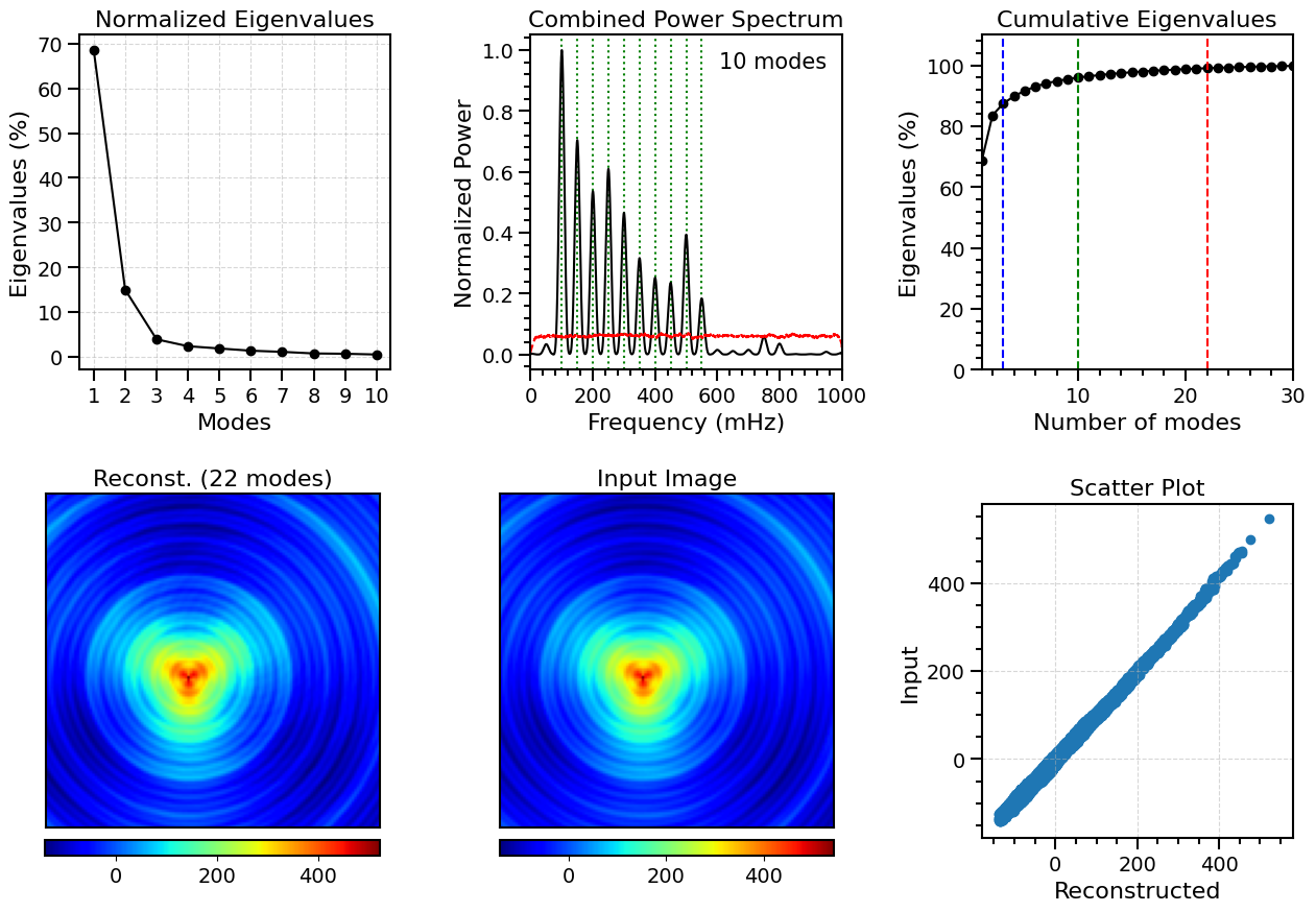
The figure below summarizes the POD analysis results, including the normalized eigenvalues, combined power spectrum, and cumulative explained variance.

Methods used:

  • Proper Orthogonal Decomposition (POD)
  • Power spectrum analysis
  • Variance analysis

WaLSAtools version: 1.0

These particular analyses generate the figure below (Supplementary Figure S6 in Nature Reviews Methods Primers; copyrighted). For a full description of the datasets and the analyses performed, see the associated article. See the source code at the bottom of this page (or here on Github) for a complete analyses and the plotting routines used to generate this figure.

jpg

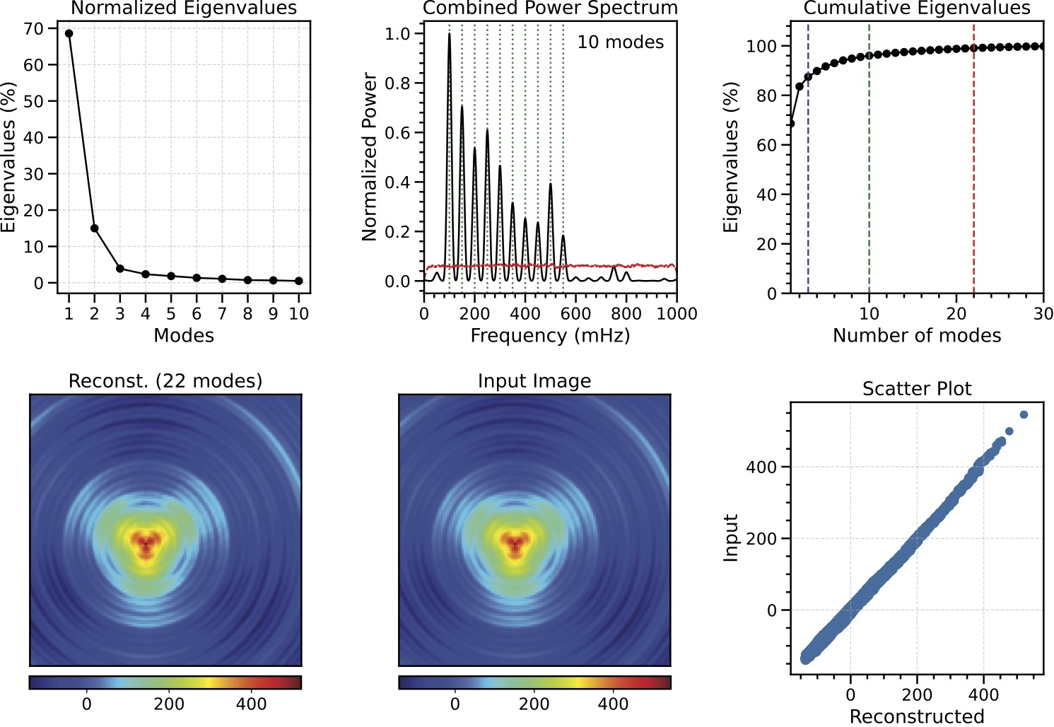
Figure Caption: POD mode analysis. Top left: Normalized squared singular values (eigenvalues) of the first ten POD modes, demonstrating their relative contributions to the total variance. Top middle: Combined power spectrum of the first ten POD modes, revealing the dominant frequencies captured by these ten modes. The vertical dotted lines mark the ten base frequencies used to construct the synthetic data; the red dashed line identifies the 95% confidence level (estimated from 1000 bootstrap resamples). Top right: Cumulative explained variance as a function of the number of POD modes included, with vertical lines indicating the cumulative variance captured by 2 (blue), 10 (green), and 22 (red) modes. Bottom left: Reconstructed image (130×130 pixels2) of the first frame of the time series using the first 22 modes. Bottom middle: Original image (130×130 pixels2; first frame) of the datacube. Bottom right: Scatter plot of the reconstructed and original image.

Source code

© 2025 WaLSA Team - Shahin Jafarzadeh et al.

This notebook is part of the WaLSAtools package (v1.0), provided under the Apache License, Version 2.0.

You may use, modify, and distribute this notebook and its contents under the terms of the license.


Important Note on Figures: Figures generated using this notebook that are identical to or derivative of those published in:
Jafarzadeh, S., Jess, D. B., Stangalini, M. et al. 2025, Nature Reviews Methods Primers, in press,
are copyrighted by Nature Reviews Methods Primers. Any reuse of such figures requires explicit permission from the journal.

Figures that are newly created, modified, or unrelated to the published article may be used under the terms of the Apache License.


Disclaimer: This notebook and its code are provided "as is", without warranty of any kind, express or implied. Refer to the license for more details.

 1
 2
 3
 4
 5
 6
 7
 8
 9
10
11
12
13
14
15
16
17
18
19
20
21
from astropy.io import fits
from WaLSAtools import WaLSAtools, WaLSA_save_pdf

# Load FITS data
data_dir = 'Synthetic_Data/'
hdul = fits.open(data_dir + 'NRMP_signal_3D.fits')
signal_3d = hdul[0].data  # 3D synthetic data
time = hdul[1].data # Time array, saved in the second HDU (Extension HDU 1)
hdul.close()

# Computed POD modes using WaLSAtools
pod_results = WaLSAtools(
    signal=signal_3d, 
    time=time, 
    method='pod', 
    num_modes=10, 
    num_top_frequencies=10, 
    num_cumulative_modes=50, 
    timestep_to_reconstruct=1,
    num_modes_reconstruct=22
)

Starting POD analysis ....
Processing a 3D cube with shape (200, 130, 130).
POD analysis completed.
Top 10 frequencies and normalized power values:
[[0.1, 1.0], [0.15, 0.7], [0.25, 0.61], [0.2, 0.54], [0.3, 0.47], [0.5, 0.39], [0.35, 0.32], [0.4, 0.25], [0.45, 0.24], [0.55, 0.18]]
Total variance contribution of the first 10 modes: 96.01%

---- POD/SPOD Results Summary ----

input_data (ndarray, Shape: (200, 130, 130)): Original input data, mean subtracted (Shape: (Nt, Ny, Nx))
spatial_mode (ndarray, Shape: (200, 130, 130)): Reshaped spatial modes matching the dimensions of the input data (Shape: (Nmodes, Ny, Nx))
temporal_coefficient (ndarray, Shape: (200, 200)): Temporal coefficients associated with each spatial mode (Shape: (Nmodes, Nt))
eigenvalue (ndarray, Shape: (200,)): Eigenvalues corresponding to singular values squared (Shape: (Nmodes))
eigenvalue_contribution (ndarray, Shape: (200,)): Eigenvalue contribution of each mode (Shape: (Nmodes))
cumulative_eigenvalues (list, Shape: (50,)): Cumulative percentage of eigenvalues for the first "num_cumulative_modes" modes (Shape: (num_cumulative_modes))
combined_welch_psd (ndarray, Shape: (8193,)): Combined Welch power spectral density for the temporal coefficients of the firts "num_modes" modes (Shape: (Nf))
frequencies (ndarray, Shape: (8193,)): Frequencies identified in the Welch spectrum (Shape: (Nf))
combined_welch_significance (ndarray, Shape: (8193,)): Significance threshold of the combined Welch spectrum (Shape: (Nf,))
reconstructed (ndarray, Shape: (130, 130)): Reconstructed frame at the specified timestep using the top "num_modes" modes (Shape: (Ny, Nx))
sorted_frequencies (ndarray, Shape: (21,)): Frequencies identified in the Welch combined power spectrum (Shape: (Nfrequencies))
frequency_filtered_modes (ndarray, Shape: (200, 130, 130, 10)): Frequency-filtered spatial POD modes for the first "num_top_frequencies" frequencies (Shape: (Nt, Ny, Nx, num_top_frequencies))
frequency_filtered_modes_frequencies (ndarray, Shape: (10,)): Frequencies corresponding to the frequency-filtered modes (Shape: (num_top_frequencies))
SPOD_spatial_modes (NoneType, Shape: None): SPOD spatial modes if SPOD is used (Shape: (Nspod_modes, Ny, Nx))
SPOD_temporal_coefficients (NoneType, Shape: None): SPOD temporal coefficients if SPOD is used (Shape: (Nspod_modes, Nt))
p (ndarray, Shape: (16900, 200)): Left singular vectors (spatial modes) from SVD (Shape: (Nx, Nmodes))
s (ndarray, Shape: (200,)): Singular values from SVD (Shape: (Nmodes))
a (ndarray, Shape: (200, 200)): Right singular vectors (temporal coefficients) from SVD (Shape: (Nmodes, Nt))


1
2
3
4
5
6
7
input_data = pod_results['input_data']
eigenvalue_contribution = pod_results['eigenvalue_contribution']
combined_welch_psd = pod_results['combined_welch_psd']
frequencies = pod_results['frequencies']
combined_welch_significance = pod_results['combined_welch_significance']
cumulative_eigenvalues = pod_results['cumulative_eigenvalues']
reconstructed = pod_results['reconstructed']
  1
  2
  3
  4
  5
  6
  7
  8
  9
 10
 11
 12
 13
 14
 15
 16
 17
 18
 19
 20
 21
 22
 23
 24
 25
 26
 27
 28
 29
 30
 31
 32
 33
 34
 35
 36
 37
 38
 39
 40
 41
 42
 43
 44
 45
 46
 47
 48
 49
 50
 51
 52
 53
 54
 55
 56
 57
 58
 59
 60
 61
 62
 63
 64
 65
 66
 67
 68
 69
 70
 71
 72
 73
 74
 75
 76
 77
 78
 79
 80
 81
 82
 83
 84
 85
 86
 87
 88
 89
 90
 91
 92
 93
 94
 95
 96
 97
 98
 99
100
101
102
103
104
105
106
107
108
109
110
111
112
113
114
115
116
117
118
119
120
121
122
123
124
125
126
127
128
129
130
131
132
133
134
135
136
137
import numpy as np
import matplotlib.pyplot as plt
import matplotlib.gridspec as gridspec 
from matplotlib.ticker import AutoMinorLocator
import matplotlib.ticker as ticker
from matplotlib.ticker import MaxNLocator

# Setting global parameters for the plots
plt.rcParams.update({
    'font.size': 14,          # Global font size
    'axes.titlesize': 16,     # Title font size
    'axes.labelsize': 16,     # Axis label font size
    'xtick.labelsize': 14,    # X-axis tick label font size
    'ytick.labelsize': 14,    # Y-axis tick label font size
    'legend.fontsize': 14,    # Legend font size
    'figure.titlesize': 17,   # Figure title font size
    'axes.grid': False,       # Turn off grid by default
    'grid.alpha': 0.5,        # Grid transparency
    'grid.linestyle': '--',   # Grid line style
})

fig = plt.figure(figsize=(15, 10))

# Create subplots with GridSpec
gs1 = gridspec.GridSpec(2, 3, figure=fig, wspace=0.45, hspace=0.4)

# Plot normalized eigenvalues
ax_ev = plt.subplot(gs1[0, 0])
ax_ev.set_title(f'Normalized Eigenvalues')
mode_nums = np.arange(1,11)
ax_ev.plot(mode_nums, 100*eigenvalue_contribution[0:10],'k-o')
ax_ev.set_xlabel('Modes')
ax_ev.set_ylabel('Eigenvalues (%)')
ax_ev.grid(True)
ax_ev.xaxis.set_major_locator(ticker.MultipleLocator(1))
ax_ev.tick_params(axis='both', which='major', direction='out', length=8, width=1.5)
ax_ev.tick_params(axis='both', labelsize=14)
for spine in ax_ev.spines.values():
    spine.set_linewidth(1.5)

# Plot combined power spectrum
ax_freq = plt.subplot(gs1[0, 1])
pre_defined_freq = [100,150,200,250,300,350,400,450,500,550]
for freq in pre_defined_freq:
    ax_freq.axvline(x=freq, color='green', linestyle=':', linewidth=1.5)
ax_freq.plot(frequencies*1000.,combined_welch_psd/np.max(combined_welch_psd),'k')
ax_freq.plot(frequencies*1000., combined_welch_significance, 'r--', label='95% Significance Threshold')
ax_freq.set_title(f'Combined Power Spectrum')
ax_freq.set_xlabel('Frequency (mHz)')
ax_freq.set_ylabel('Normalized Power')
ax_freq.grid(False)
ax_freq.xaxis.set_minor_locator(AutoMinorLocator(5))
ax_freq.yaxis.set_minor_locator(AutoMinorLocator(5))
ax_freq.tick_params(axis='both', which='major', direction='out', length=8, width=1.5)
ax_freq.tick_params(axis='both', which='minor', direction='out', length=4, width=1.5)
ax_freq.tick_params(axis='both', labelsize=14)
for spine in ax_freq.spines.values():
    spine.set_linewidth(1.5)
ax_freq.set_xlim(0,1000)
ax_freq.text(0.95, 0.95, '10 modes', transform=ax_freq.transAxes, fontsize=15, verticalalignment='top', horizontalalignment='right')

# Plot cumulative eigenvalues
ax_freq = plt.subplot(gs1[0, 2])
ax_freq.plot(cumulative_eigenvalues,'k-o')
ax_freq.set_title(f'Cumulative Eigenvalues')
ax_freq.set_xlabel('Number of modes')
ax_freq.set_ylabel('Eigenvalues (%)')
ax_freq.grid(False)
ax_freq.xaxis.set_minor_locator(AutoMinorLocator(5))
ax_freq.yaxis.set_minor_locator(AutoMinorLocator(5))
ax_freq.tick_params(axis='both', which='major', direction='out', length=8, width=1.5)
ax_freq.tick_params(axis='both', which='minor', direction='out', length=4, width=1.5)
ax_freq.tick_params(axis='both', labelsize=14)
for spine in ax_freq.spines.values():
    spine.set_linewidth(1.5)
ax_freq.set_xlim(1,30)
ax_freq.set_ylim(0,110)

# Identify indices where 90% and 95% is reached
thresholds = [84, 96, 99]
colors = ['blue', 'green', 'red']
for threshold, color in zip(thresholds, colors):
    index = next(i for i, v in enumerate(cumulative_eigenvalues) if v >= threshold)
    ax_freq.axvline(x=index, color=color, linestyle='--', label=f'{threshold}% at mode {index}')

# Plot reconstructed image for frame number 1 (using the first 22 modes)
im_recon = plt.subplot(gs1[1, 0])
im_recon.set_title('Reconst. (22 modes)')
img = im_recon.imshow(reconstructed, cmap='jet', aspect='equal', origin='lower')
im_recon.set_xticks([])  # Remove x ticks
im_recon.set_yticks([])  # Remove y ticks
for spine in im_recon.spines.values():
        spine.set_linewidth(1.5)
im_recon.set_position([0.05, 0.12, 0.32, 0.32])  # Adjust these values (left, bottom, width, height)
# Create a new axis for the colorbar and set its position
cax = fig.add_axes([0.103, 0.093, 0.2135, 0.015])  # Adjust these values (left, bottom, width, height)
colorbar = plt.colorbar(img, cax=cax, orientation='horizontal')
colorbar.outline.set_linewidth(1.5)

# Plot input image (mean subtracted) for frame number 1 
im_input = plt.subplot(gs1[1, 1])
im_input.set_title('Input Image')
img2 = im_input.imshow(input_data[1, :, :], cmap='jet', aspect='equal', origin='lower')
im_input.set_xticks([])  # Remove x ticks
im_input.set_yticks([])  # Remove y ticks
for spine in im_input.spines.values():
        spine.set_linewidth(1.5)
im_input.set_position([0.34, 0.12, 0.32, 0.32])  # Adjust these values (left, bottom, width, height)
# Create a new axis for the colorbar and set its position
cax2 = fig.add_axes([0.3935, 0.093, 0.2135, 0.015])  # Adjust these values (left, bottom, width, height)
colorbar = plt.colorbar(img2, cax=cax2, orientation='horizontal')
colorbar.outline.set_linewidth(1.5)

# Add scatter plot
ax_scatter = plt.subplot(gs1[1, 2])
ax_scatter.set_title('Scatter Plot')
ax_scatter.scatter(reconstructed, input_data[1, :, :])
ax_scatter.set_xlabel('Reconstructed')
ax_scatter.set_ylabel('Input')
ax_scatter.grid(True)
ax_scatter.xaxis.set_minor_locator(AutoMinorLocator(4))
ax_scatter.yaxis.set_minor_locator(AutoMinorLocator(4))
ax_scatter.xaxis.set_major_locator(MaxNLocator(nbins=4))
ax_scatter.yaxis.set_major_locator(MaxNLocator(nbins=4))
ax_scatter.tick_params(axis='both', which='major', direction='out', length=8, width=1.5)
ax_scatter.tick_params(axis='both', which='minor', direction='out', length=4, width=1.5)
ax_scatter.tick_params(axis='both', labelsize=14)
for spine in ax_scatter.spines.values():
    spine.set_linewidth(1.5)
ax_scatter.set_xlim(-180,580)
ax_scatter.set_ylim(-180,580)

# Save the figure as a PDF
pdf_path = 'Figures/FigS6_POD_eigenvalues_powerspectrum.pdf'
WaLSA_save_pdf(fig, pdf_path, color_mode='CMYK', dpi=300, bbox_inches='tight', pad_inches=0)

plt.show()

GPL Ghostscript 10.04.0 (2024-09-18)
Copyright (C) 2024 Artifex Software, Inc. All rights reserved.
This software is supplied under the GNU AGPLv3 and comes with NO WARRANTY:
see the file COPYING for details.
Processing pages 1 through 1.
Page 1
PDF saved in CMYK format as 'Figures/FigS6_POD_egenvalues_powerspectrum.pdf'

png