Skip to content

Worked Example - NRMP: POD with Frequency Filtering

This example demonstrates the application of frequency filtering to the temporal coefficients of POD modes. By isolating specific frequencies in the temporal evolution of each mode, we can extract spatial patterns associated with those frequencies, revealing more detailed information about the wave behaviour.

Analysis and Figure

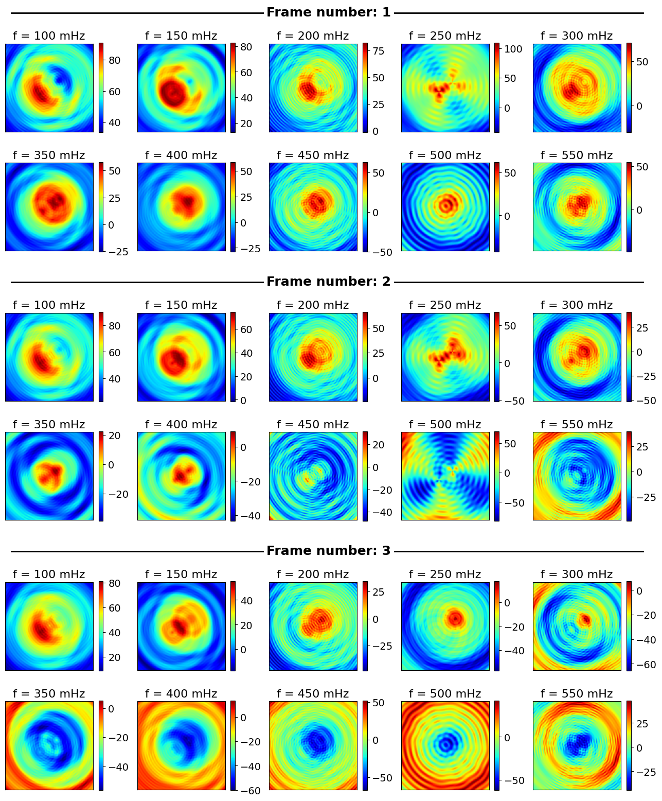
The figure below shows the frequency-filtered spatial modes for the ten dominant frequencies in the synthetic spatio-temporal dataset.

Methods used:

  • Proper Orthogonal Decomposition (POD)
  • Frequency filtering of temporal coefficients

WaLSAtools version: 1.0

These particular analyses generate the figure below (Supplementary Figure S7 in Nature Reviews Methods Primers; copyrighted). For a full description of the datasets and the analyses performed, see the associated article. See the source code at the bottom of this page (or here on Github) for a complete analyses and the plotting routines used to generate this figure.

jpg

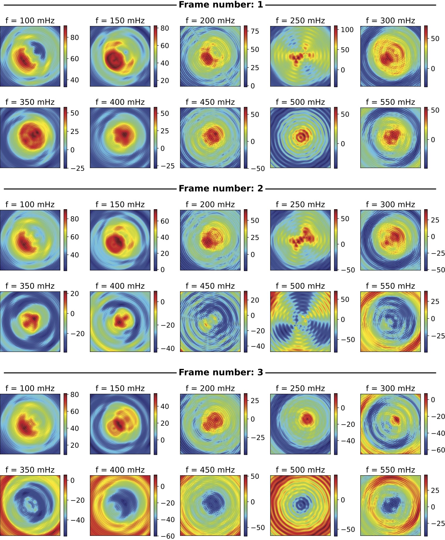
Figure Caption: Frequency-filtered spatial modes for the ten dominant frequencies. The spatial patterns associated with each frequency are shown for the first three time steps of the series, with each image covering 130×130 pixels2.

Source code

© 2025 WaLSA Team - Shahin Jafarzadeh et al.

This notebook is part of the WaLSAtools package (v1.0), provided under the Apache License, Version 2.0.

You may use, modify, and distribute this notebook and its contents under the terms of the license.


Important Note on Figures: Figures generated using this notebook that are identical to or derivative of those published in:
Jafarzadeh, S., Jess, D. B., Stangalini, M. et al. 2025, Nature Reviews Methods Primers, in press,
are copyrighted by Nature Reviews Methods Primers. Any reuse of such figures requires explicit permission from the journal.

Figures that are newly created, modified, or unrelated to the published article may be used under the terms of the Apache License.


Disclaimer: This notebook and its code are provided "as is", without warranty of any kind, express or implied. Refer to the license for more details.

 1
 2
 3
 4
 5
 6
 7
 8
 9
10
11
12
13
14
15
16
17
18
19
20
21
22
from astropy.io import fits
from WaLSAtools import WaLSAtools, WaLSA_save_pdf

# Load FITS data
data_dir = 'Synthetic_Data/'
hdul = fits.open(data_dir + 'NRMP_signal_3D.fits')
signal_3d = hdul[0].data  # 3D synthetic data
time = hdul[1].data # Time array, saved in the second HDU (Extension HDU 1)
hdul.close()

# Computed POD modes using WaLSAtools
pod_results = WaLSAtools(
    signal=signal_3d, 
    time=time, 
    method='pod', 
    num_modes=10, 
    num_top_frequencies=10, 
    top_frequencies = [0.10, 0.15, 0.20, 0.25, 0.30, 0.35, 0.40, 0.45, 0.50, 0.55], # in Hz
    num_cumulative_modes=50, 
    timestep_to_reconstruct=1,
    num_modes_reconstruct=22  
)

Starting POD analysis ....
Processing a 3D cube with shape (200, 130, 130).
POD analysis completed.
Top 10 frequencies and normalized power values:
[[0.1, 1.0], [0.15, 0.7], [0.25, 0.61], [0.2, 0.54], [0.3, 0.47], [0.5, 0.39], [0.35, 0.32], [0.4, 0.25], [0.45, 0.24], [0.55, 0.18]]
Total variance contribution of the first 10 modes: 96.01%

---- POD/SPOD Results Summary ----

input_data (ndarray, Shape: (200, 130, 130)): Original input data, mean subtracted (Shape: (Nt, Ny, Nx))
spatial_mode (ndarray, Shape: (200, 130, 130)): Reshaped spatial modes matching the dimensions of the input data (Shape: (Nmodes, Ny, Nx))
temporal_coefficient (ndarray, Shape: (200, 200)): Temporal coefficients associated with each spatial mode (Shape: (Nmodes, Nt))
eigenvalue (ndarray, Shape: (200,)): Eigenvalues corresponding to singular values squared (Shape: (Nmodes))
eigenvalue_contribution (ndarray, Shape: (200,)): Eigenvalue contribution of each mode (Shape: (Nmodes))
cumulative_eigenvalues (list, Shape: (50,)): Cumulative percentage of eigenvalues for the first "num_cumulative_modes" modes (Shape: (num_cumulative_modes))
combined_welch_psd (ndarray, Shape: (8193,)): Combined Welch power spectral density for the temporal coefficients of the firts "num_modes" modes (Shape: (Nf))
frequencies (ndarray, Shape: (8193,)): Frequencies identified in the Welch spectrum (Shape: (Nf))
combined_welch_significance (ndarray, Shape: (8193,)): Significance threshold of the combined Welch spectrum (Shape: (Nf,))
reconstructed (ndarray, Shape: (130, 130)): Reconstructed frame at the specified timestep using the top "num_modes" modes (Shape: (Ny, Nx))
sorted_frequencies (ndarray, Shape: (21,)): Frequencies identified in the Welch combined power spectrum (Shape: (Nfrequencies))
frequency_filtered_modes (ndarray, Shape: (200, 130, 130, 10)): Frequency-filtered spatial POD modes for the first "num_top_frequencies" frequencies (Shape: (Nt, Ny, Nx, num_top_frequencies))
frequency_filtered_modes_frequencies (list, Shape: (10,)): Frequencies corresponding to the frequency-filtered modes (Shape: (num_top_frequencies))
SPOD_spatial_modes (NoneType, Shape: None): SPOD spatial modes if SPOD is used (Shape: (Nspod_modes, Ny, Nx))
SPOD_temporal_coefficients (NoneType, Shape: None): SPOD temporal coefficients if SPOD is used (Shape: (Nspod_modes, Nt))
p (ndarray, Shape: (16900, 200)): Left singular vectors (spatial modes) from SVD (Shape: (Nx, Nmodes))
s (ndarray, Shape: (200,)): Singular values from SVD (Shape: (Nmodes))
a (ndarray, Shape: (200, 200)): Right singular vectors (temporal coefficients) from SVD (Shape: (Nmodes, Nt))


1
2
frequency_filtered_modes = pod_results['frequency_filtered_modes']
frequency_filtered_modes_frequencies = pod_results['frequency_filtered_modes_frequencies']
  1
  2
  3
  4
  5
  6
  7
  8
  9
 10
 11
 12
 13
 14
 15
 16
 17
 18
 19
 20
 21
 22
 23
 24
 25
 26
 27
 28
 29
 30
 31
 32
 33
 34
 35
 36
 37
 38
 39
 40
 41
 42
 43
 44
 45
 46
 47
 48
 49
 50
 51
 52
 53
 54
 55
 56
 57
 58
 59
 60
 61
 62
 63
 64
 65
 66
 67
 68
 69
 70
 71
 72
 73
 74
 75
 76
 77
 78
 79
 80
 81
 82
 83
 84
 85
 86
 87
 88
 89
 90
 91
 92
 93
 94
 95
 96
 97
 98
 99
100
101
102
103
104
105
106
107
108
109
110
import numpy as np
import matplotlib.pyplot as plt
import matplotlib.gridspec as gridspec 

# Setting global parameters for the plot
plt.rcParams.update({
    'font.size': 14,          # Global font size
    'axes.titlesize': 16,     # Title font size
    'axes.labelsize': 16,     # Axis label font size
    'xtick.labelsize': 12,    # X-axis tick label font size
    'ytick.labelsize': 12,    # Y-axis tick label font size
    'legend.fontsize': 14,    # Legend font size
    'figure.titlesize': 17,   # Figure title font size
    'axes.grid': False,       # Turn off grid by default
    'grid.alpha': 0.5,        # Grid transparency
    'grid.linestyle': '--',   # Grid line style
})

figure = plt.figure(figsize=(16., 20.))  # Set figure size
gs1 = gridspec.GridSpec(9, 5, figure=figure, height_ratios=[0.15, 1, 1, 0.15, 1, 1, 0.15, 1, 1])

# Add a horizontal line and title (frame number)
line_ax1 = plt.subplot(gs1[0, :])
line_ax1.plot([0.01, 1], [0, 0], clip_on=False, color='black', linewidth=2)
plt.text(0.41, 0, 'Frame number: 1', fontsize=18, fontweight='bold', verticalalignment='center', bbox=dict(facecolor='white', edgecolor='none'))
line_ax1.axis('off')
line_ax1.set_xticks([])  # Remove x ticks
line_ax1.set_yticks([])  # Remove y ticks
line_ax1.set_xlim(0, 1)

frame_index = 0
for i in range(0, 5):
    ax_img = plt.subplot(gs1[1, i])
    img = plt.imshow(frequency_filtered_modes[frame_index, :, :, i], cmap='jet', aspect='equal', origin='lower')
    ax_img.set_title(f'f = {(int(np.round(frequency_filtered_modes_frequencies[i]*1000)))} mHz')
    ax_img.set_xticks([])  # Remove x ticks
    ax_img.set_yticks([])  # Remove y ticks
    cbar = plt.colorbar(img, orientation='vertical', shrink=0.86)
    cbar.ax.tick_params(labelsize=14)

for j in range(5, 10):
    ax_img = plt.subplot(gs1[2, j-5])
    img = plt.imshow(frequency_filtered_modes[frame_index, :, :, j], cmap='jet', aspect='equal', origin='lower')
    ax_img.set_title(f'f = {(int(np.round(frequency_filtered_modes_frequencies[j]*1000)))} mHz')
    ax_img.set_xticks([])  # Remove x ticks
    ax_img.set_yticks([])  # Remove y ticks
    cbar = plt.colorbar(img, orientation='vertical', shrink=0.86)
    cbar.ax.tick_params(labelsize=14)

# Add a horizontal line and title (frame number)
line_ax1 = plt.subplot(gs1[3, :])
line_ax1.plot([0.01, 1], [0, 0], clip_on=False, color='black', linewidth=2)
plt.text(0.41, 0, 'Frame number: 2', fontsize=18, fontweight='bold', verticalalignment='center', bbox=dict(facecolor='white', edgecolor='none'))
line_ax1.axis('off')
line_ax1.set_xticks([])  # Remove x ticks
line_ax1.set_yticks([])  # Remove y ticks
line_ax1.set_xlim(0, 1)

frame_index = 1
for i in range(0, 5):
    ax_img = plt.subplot(gs1[4, i])
    img = plt.imshow(frequency_filtered_modes[frame_index, :, :, i], cmap='jet', aspect='equal', origin='lower')
    ax_img.set_title(f'f = {(int(np.round(frequency_filtered_modes_frequencies[i]*1000)))} mHz')
    ax_img.set_xticks([])  # Remove x ticks
    ax_img.set_yticks([])  # Remove y ticks
    cbar = plt.colorbar(img, orientation='vertical', shrink=0.86)
    cbar.ax.tick_params(labelsize=14)

for j in range(5, 10):
    ax_img = plt.subplot(gs1[5, j-5])
    img = plt.imshow(frequency_filtered_modes[frame_index, :, :, j], cmap='jet', aspect='equal', origin='lower')
    ax_img.set_title(f'f = {(int(np.round(frequency_filtered_modes_frequencies[j]*1000)))} mHz')
    ax_img.set_xticks([])  # Remove x ticks
    ax_img.set_yticks([])  # Remove y ticks
    cbar = plt.colorbar(img, orientation='vertical', shrink=0.86)
    cbar.ax.tick_params(labelsize=14)

# Add a horizontal line and title (frame number)
line_ax1 = plt.subplot(gs1[6, :])
line_ax1.plot([0.01, 1], [0, 0], clip_on=False, color='black', linewidth=2)
plt.text(0.41, 0, 'Frame number: 3', fontsize=18, fontweight='bold', verticalalignment='center', bbox=dict(facecolor='white', edgecolor='none'))
line_ax1.axis('off')
line_ax1.set_xticks([])  # Remove x ticks
line_ax1.set_yticks([])  # Remove y ticks
line_ax1.set_xlim(0, 1)

frame_index = 2
for i in range(0, 5):
    ax_img = plt.subplot(gs1[7, i])
    img = plt.imshow(frequency_filtered_modes[frame_index, :, :, i], cmap='jet', aspect='equal', origin='lower')
    ax_img.set_title(f'f = {(int(np.round(frequency_filtered_modes_frequencies[i]*1000)))} mHz')
    ax_img.set_xticks([])  # Remove x ticks
    ax_img.set_yticks([])  # Remove y ticks
    cbar = plt.colorbar(img, orientation='vertical', shrink=0.86)
    cbar.ax.tick_params(labelsize=14)

for j in range(5, 10):
    ax_img = plt.subplot(gs1[8, j-5])
    img = plt.imshow(frequency_filtered_modes[frame_index, :, :, j], cmap='jet', aspect='equal', origin='lower')
    ax_img.set_title(f'f = {(int(np.round(frequency_filtered_modes_frequencies[j]*1000)))} mHz')
    ax_img.set_xticks([])  # Remove x ticks
    ax_img.set_yticks([])  # Remove y ticks
    cbar = plt.colorbar(img, orientation='vertical', shrink=0.86)
    cbar.ax.tick_params(labelsize=14)

# Save the figure as a PDF
pdf_path = 'Figures/FigS7_POD_frequency_filtered_spatial_modes.pdf'
WaLSA_save_pdf(figure, pdf_path, color_mode='CMYK', dpi=300, bbox_inches='tight', pad_inches=0)

plt.show()

GPL Ghostscript 10.04.0 (2024-09-18)
Copyright (C) 2024 Artifex Software, Inc. All rights reserved.
This software is supplied under the GNU AGPLv3 and comes with NO WARRANTY:
see the file COPYING for details.
Processing pages 1 through 1.
Page 1
PDF saved in CMYK format as 'Figures/FigS7_POD_frequency_filtered_spatial_modes.pdf'

png

 1
 2
 3
 4
 5
 6
 7
 8
 9
10
# Save the first six frames of the frequency-filtered POD reconstruction at 0.5 Hz (500 mHz), as a FITS file.
# To be used in Figure 5 of the Nature Reviews Methods Primers paper

num_images = 6
freq_index = np.where(np.isclose(frequency_filtered_modes_frequencies, 0.5))[0]
data_cube = np.zeros((num_images, signal_3d.shape[1], signal_3d.shape[2]))
for i in range(num_images):
    data_cube[i, :, :] = frequency_filtered_modes[i, :, :, freq_index]
hdu_var = fits.PrimaryHDU(data_cube)
hdu_var.writeto('Saved_Parameters/POD_first_6_frequency_filtered_spatial_modes_at_500mHz.fits', overwrite=True)
 1
 2
 3
 4
 5
 6
 7
 8
 9
10
11
12
13
14
15
16
17
18
19
20
21
22
23
24
25
26
27
28
29
30
31
32
33
34
35
36
37
38
39
40
41
42
43
44
45
46
47
48
49
50
# Create a set of images for the frequency-filtered POD reconstruction at all time steps
# To be used in the Supplementary Video 2

# Setting global parameters
plt.rcParams.update({
    'font.size': 14,          # Global font size
    'axes.titlesize': 16,     # Title font size
    'axes.labelsize': 16,     # Axis label font size
    'xtick.labelsize': 12,    # X-axis tick label font size
    'ytick.labelsize': 12,    # Y-axis tick label font size
    'legend.fontsize': 14,    # Legend font size
    'figure.titlesize': 17,   # Figure title font size
    'axes.grid': False,        # Turn on grid by default
    'grid.alpha': 0.5,        # Grid transparency
    'grid.linestyle': '--',   # Grid line style
})

for frame_index in range(0, 200):
    figure = plt.figure(figsize=(16., 6.6))
    gs1 = gridspec.GridSpec(5, 5, figure=figure, height_ratios=[0.1, 0.1, 1, 0.1, 1])

    # Add a horizontal line and title (frame number)
    line_ax1 = plt.subplot(gs1[0, :])
    line_ax1.plot([0.01, 1], [0, 0], clip_on=False, color='black', linewidth=2)
    plt.text(0.405, 0, f'Frame number: {frame_index+1}', fontsize=18, fontweight='bold', verticalalignment='center', bbox=dict(facecolor='white', edgecolor='none'))
    line_ax1.axis('off')
    line_ax1.set_xticks([])  # Remove x ticks
    line_ax1.set_yticks([])  # Remove y ticks
    line_ax1.set_xlim(0,1)

    for i in range(0, 5):
        ax_img = plt.subplot(gs1[2, i])
        img = plt.imshow(frequency_filtered_modes[frame_index, :, :, i], cmap='jet', aspect='equal', origin='lower')
        ax_img.set_title(f'f = {(int(np.round(frequency_filtered_modes_frequencies[i]*1000)))} mHz')
        ax_img.set_xticks([])  # Remove x ticks
        ax_img.set_yticks([])  # Remove y ticks
        cbar.ax.tick_params(labelsize=14)

    for j in range(5, 10):
        ax_img = plt.subplot(gs1[4, j-5])
        img = plt.imshow(frequency_filtered_modes[frame_index, :, :, j], cmap='jet', aspect='equal', origin='lower')
        ax_img.set_title(f'f = {(int(np.round(frequency_filtered_modes_frequencies[j]*1000)))} mHz')
        ax_img.set_xticks([])  # Remove x ticks
        ax_img.set_yticks([])  # Remove y ticks
        cbar.ax.tick_params(labelsize=14)

    plt.savefig(f'Video_Snapshots/POD_spectral_images__video_S2/im_{frame_index:03d}.jpg', dpi=300, bbox_inches='tight', pad_inches=0.2)  
    plt.close()

print("Images saved successfully.")

Images saved successfully.